semi合集-English.pdf - 第7567页
SEMI MF1811-0704 © SEMI 2003, 2004 14 random num b er generat or correspon d ing to a const ant PSD and are not the results of an actual measurem ent. In addition, the number of data points has been limited to N = 32 and…

SEMI MF1811-0704 © SEMI 2003, 2004 13
5.5 Periodogram Estimators of the Rms Profile
Roughness and Slope
5.5.1 The periodogram estimator of the rms profile
height, ,
q
R
)
is as follows:
∑
+
=
=
)2/(1
2
1
)(
1
N
m
q
mS
ND
R
)
)
(35)
This quantity has the same dimension as the original
height measurements and is independent of the
magnitude and dimensions of the sampling interval, D.
5.5.2 The corresponding estimator for the rms profile
slope, ,
q
∆
)
is as follows:
∑∑
+
=
+
=
−π=
′
=∆
)2/(1
2
1
2
3
)2/(1
2
1
)()1(
)(
1
2)(
1
N
m
N
m
q
mSm
ND
mS
ND
))
)
(36)
In evaluating these quantities the height measurements,
Z, and the sampling interval, D, must be expressed in
the same length units. Although
q
∆
)
is in units of
radians, its magnitude scales as 1/D.
5.6 Window Functions
5.6.1 Window functions appear in a wide variety of
signal-processing applications, with different shapes
and normalizations. Although this guide recommends
the use of the Hann or Blackman window, other forms
are included for comparison. All are normalized so that
∑
=
=
N
n
nW
N
1
2
1)(
1
in order to preserve the magnitudes of
average values of the mean-square profile statistics.
5.6.2 Particular forms are:
5.6.2.1 Rectangular or Daniell window:
1)( =nW (37)
5.6.2.2 Hann, or Raised Cosine window:
−π
−=
N
n
nW
)1(2
cos124
1728
2
)(
(38)
5.6.2.3 Hamming window:
−π
−⋅=
N
n
nW
)1(2
cos2327
1987
2
)(
(39)
5.6.2.4 Blackman window:
−π
+
−π
−⋅=
N
n
N
n
nW
)1(4
cos4
)1(2
cos2521
1523
2
)(
(40)
NOTE 17: The choice of window functions is of minor
importance for randomly-rough surfaces as long as it
smoothes the data at the ends of the data record. The
rectangular or Daniell window does not do this, but is useful
for numerical checking.
NOTE 18: In the case of profiles with a smooth PSD, the
principal effect the window shape is to change the fine-scale
fluctuations in the periodogram estimate without changing its
ensemble-average value, except, perhaps, near the LFL.
NOTE 19: In the case of profiles involving periodicities, the
window shape can change the shape of the sharp lines in the
PSD, albeit without changing their areas. The choice of the
window shape then involves a trade-off between line width
and smoothness. The raised Hann or Blackman windows are
recommended for general use.
NOTE 20: If the estimation routines are applied to
deterministic profiles, such as individual steps, pits, or bumps,
a data window must still be used to minimize effects of the
finite data record, but the object should be placed in the center
of the profile where the window function is relatively flat.
5.7 Zero Padding
5.7.1 The fastest FFT routines require the total number
of data points to be a power of two, such as N = 2
10
=
1024. If the number of measured points, N, is not a
power of two but lies between 2
a
and 2
b
, the power-of-
two routines can be used by dropping N−2
a
points from
one end of the original data set, or by adding 2
b
−N
zeros and replacing N in the routines everywhere by 2
b
.
5.7.2 The first method is wasteful of data, while the
second uses the full set of measured data but requires
that the estimated PSD be renormalized by multiplying
it by the factor 2
b
/N.
5.8 Averaging of Statistical Quantities:
5.8.1 Power spectral density functions, the mean-
square roughness, and slope values estimated from a
number of individual profiles that have the same
statistical properties can each be averaged together to
obtain composite results. In the case of homogeneously
and isotropically rough surfaces the profiles can lie in
any position and direction on the surface under test. In
the case of homogeneously but anisotropically rough
surfaces they can lie anywhere on the surface but must
lie parallel with each other, preferably perpendicular to
the surface axis. Averaging data lowers the errors
associated with individual measurements.
6 Numerical Test Sequences
6.1 Table 1 presents a set of numerical data for testing
the execution of the users’ implementations of
algorithms discussed in Section 5.
6.2 Although these simulated profile data are in
standard notation, they have been generated by a

SEMI MF1811-0704 © SEMI 2003, 2004 14
random number generator corresponding to a constant
PSD and are not the results of an actual measurement.
In addition, the number of data points has been limited
to N = 32 and the profile heights have been rounded to
digits with magnitudes less than 100 to simplify their
manual input into the users’ programs.
6.3 Actual measured data sets would generally involve
many more data points with height values involving a
larger number of significant digits, and with different
orders of magnitude than those used in this test
sequence.
6.4 In order to provide a means for checking the proper
inclusion of the sampling distance, D, in the spectral-
estimation routines, the value D = 0.1 has been used.
6.5 Tables 2 and 3 give the values of the periodogram
estimates of the profile power spectral density,
,)(
1
mS
)
of the data in Table 1 for the three different types of
detrending described in Section 5.1. The values of
these estimates depend on the data window used. Table
2 uses a rectangular window and Table 3 uses the
Blackman window.
6.6 The dimensions of the power spectral densities in
these tables is length-cubed = (units of Z)
2
·(units of D),
and its magnitude at a given spatial frequency scales as
the sampling interval, D.
6.7 The spatial frequency is given as follows:
ND
m
f
m
1−
= (41)
where:
m = 1 corresponds to the dc or piston part of the
profile, and
m = 1 + N/2 = 17 is the Nyquist frequency in
(units of D
–1
).
6.7.1 Note that since the window function has been
applied after the detrending process, the dc terms do not
necessarily vanish for a non-rectangular window
functions.
6.8 Table 4 gives values of
q
R
)
derived from the
spectra in Table 2 and Table 3 using the expression
given in Table 4.
6.8.1 As mentioned, the unit of
q
R
)
is the same as that
of the height measurement since the magnitude and
dimensions of the sampling interval, D, cancels out in
the evaluation of R
q
.
6.9 The data in Table 2 through Table 4 are adequate
for checking the users' implementation of the estimators
described in Section 5, and further test data are not
included in this guide.
7 Related Documents
7.1 Press, W. H., Flannery, B. P., Teukolsky, S. A., and
Vetterling, W. T., Numerical Recipes – the Art of
Scientific Computing, Cambridge University Press,
Cambridge, 1986.
7.2 Church, E. L., and Takacs, P. Z., “BASIC program
for power spectrum estimation”, Brookhaven National
Laboratory Report BNL No. 49035, May 1993 (revised
May 1994).
7.3 Stover, J. C., Optical Scattering: Measurement and
Analysis, SPIE Press, l995.
7.4 Kay, S. M. Modern Spectral Estimation;Theory
and Application, Prentice Hall, l988.
7.5 Marple, Jr., S. L., Digital Spectral Analysis with
Applications (Prentice Hall, 1987).
7.6 Harris, F. J., “On the Use of Windows for
Harmonic Analysis With the Discrete Fourier
Transform,” Proceedings IEEE 66, 51–83 (1978).
7.7 Oppenheim, A. V., and Schafer, R. W., Digital
Signal Processing, Chapter 11, Prentice Hall, l975.
7.8 Bendat, J. S., and Piersol, A. G., Random Data;
Analysis and Measurement, Chapter 9 (Wiley, l971).
7.9 Church, E. L., Vorburger, T. V., and Wyant, J. C.,
“Direct Comparison of Mechanical and Optical
Measurements of the Finish of Precision Machined and
Optical Surfaces,” Optical Engineering, 24, 388–395
(1985).
7.10 Blackman, R. B., and Tukey, J. W., The
Measurement of Power Spectra (Dover, l959).
8 Keywords
8.1 estimates; estimators; power spectral density; rms
values; root mean square; roughness; slope; surface
roughness; surface slope; surface statistics.
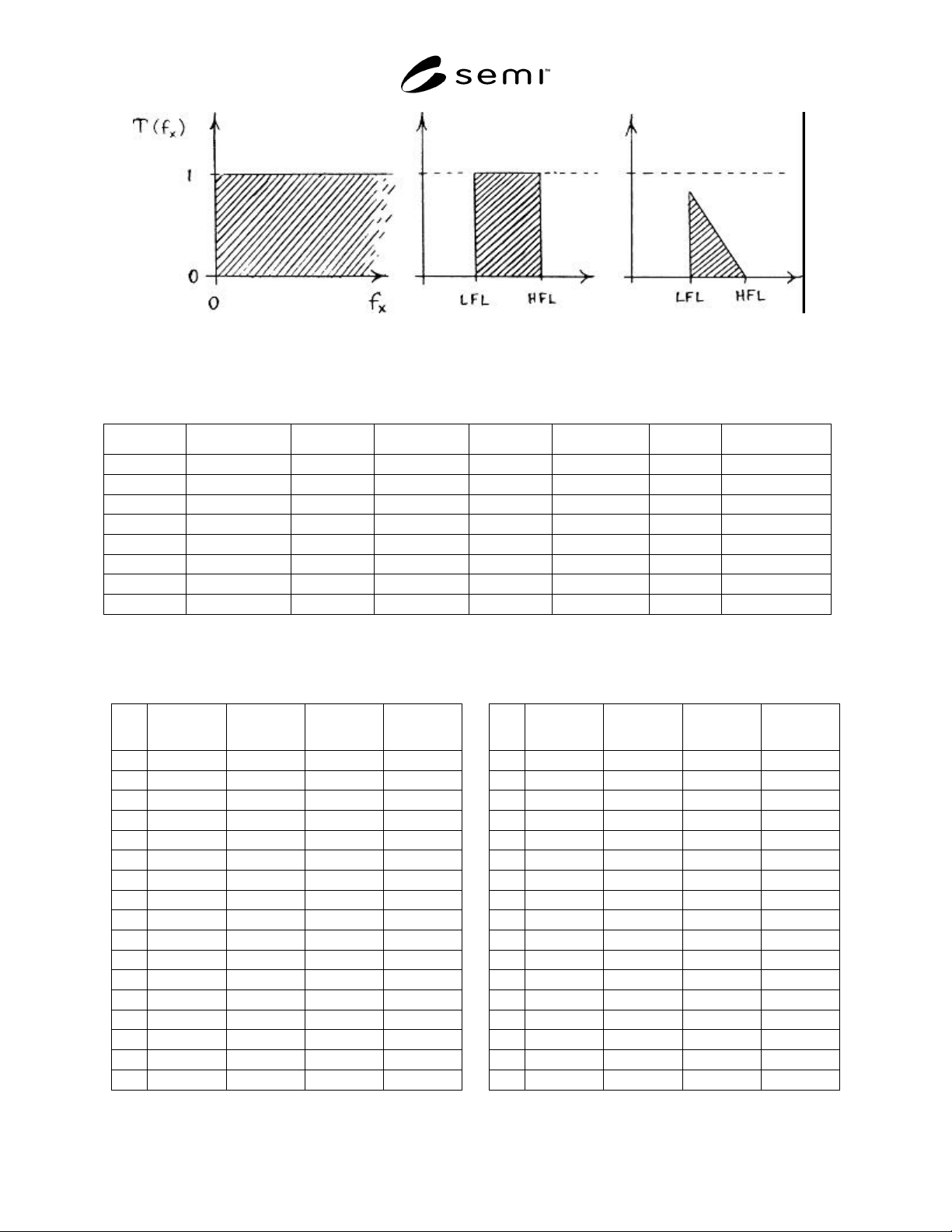
SEMI MF1811-0704 © SEMI 2003, 2004 15
Figure 1
Different Forms of the Measurement-Transfer or Instrumental-Response Function as a Function of Spatial
Frequency, f
x
.
Table 1 Simulated Height Data (N = 32)
n Z(n) n Z(n) n Z(n) n Z(n)
1 –38 9 –40 17 3 25 –35
2 15 10 45 18 6 26 23
3 36 11 20 19 17 27 4
4 22 12 3 20 20 28 –8
5 29 13 47 21 24 29 –45
6 –43 14 –18 22 16 30 26
7 –1 15 45 23 –5 31 1
8 –5 16 43 24 –17 32 6
Table 2 Periodogram Estimates (m)S
)
for Different
Types of Data Detrending Using a Rectangular
Window
m None Piston Piston+Tilt
Full
Quadratic
1 120.0500 0 0 0
2 205.9506 205.9506 182.5409 14.81781
3 142.1861 142.1861 137.3580 204.3631
4 56.98463 56.98463 44.47469 53.08546
5 147.9039 147.9039 139.6268 126.5831
6 58.60630 58.60630 55.67305 50.13899
7 248.4120 248.4120 264.7417 266.1277
8 152.8321 152.8321 158.6038 154.5160
9 185.1250 185.1250 192.8103 190.0105
10 28.81090 28.81090 26.22179 25.40131
11 28.61438 28.61438 27.90264 28.74841
12 153.1641 153.1641 145.7812 145.2367
13 356.5711 356.5711 366.4113 365.4717
14 199.1965 199.1965 202.6268 203.4514
15 41.53757 41.53757 40.26207 40.50671
16 163.6550 163.6550 168.8428 169.0258
17 16.20000 16.20000 17.87214 17.87215
Table 3 Periodogram Estimates (m)S
)
for Different
Types of Data Detrending Using a Blackman
Window
m None Piston Piston+Tilt
Full
Quadratic
1 312.4632 87.20874 90.11245 9.832211
2 536.6033 268.4217 260.2453 76.63136
3 195.1412 166.9871 162.0176 93.70938
4 1.046170 1.046172 1.041742 1.303189
5 30.14155 30.14156 30.16028 30.25176
6 54.87353 54.87350 54.91950 54.94658
7 188.9816 188.9818 188.8795 188.8293
8 74.45938 74.45934 74.50156 74.51955
9 45.28967 45.28967 45.27541 45.29324
10 59.40473 59.40471 59.41950 59.41210
11 94.24771 94.24768 94.23248 94.23342
12 202.7328 202.7328 202.7405 202.7253
13 289.7414 289.7414 289.7450 289.7637
14 130.1287 130.1287 130.1230 130.1162
15 76.22277 76.22275 76.22527 76.22248
16 62.42836 62.42840 62.42742 62.43071
17 5.585947 5.585948 5.585947 5.584926