semi合集-English.pdf - 第7202页
SEMI ME1392-0305 © SEMI 2003, 2005 11 A1-3 Receiver Geometry A1-3.1 In m any cases the field stop is set by the detector si ze; however, as the aperture stop approaches the field stop the risk of seeing unwanted stray li…
SEMI ME1392-0305 © SEMI 2003, 2005 10
APPENDIX 1
GEOMETRY
NOTICE: The material in this appendix is an official part of SEMI ME1392. It was developed during the original
approval of this standard by ASTM Committee E12 in 1996. SEMI approval was by full letter ballot procedures
with publication authorized by the NA Regional Standards Committee on December 10, 2004.
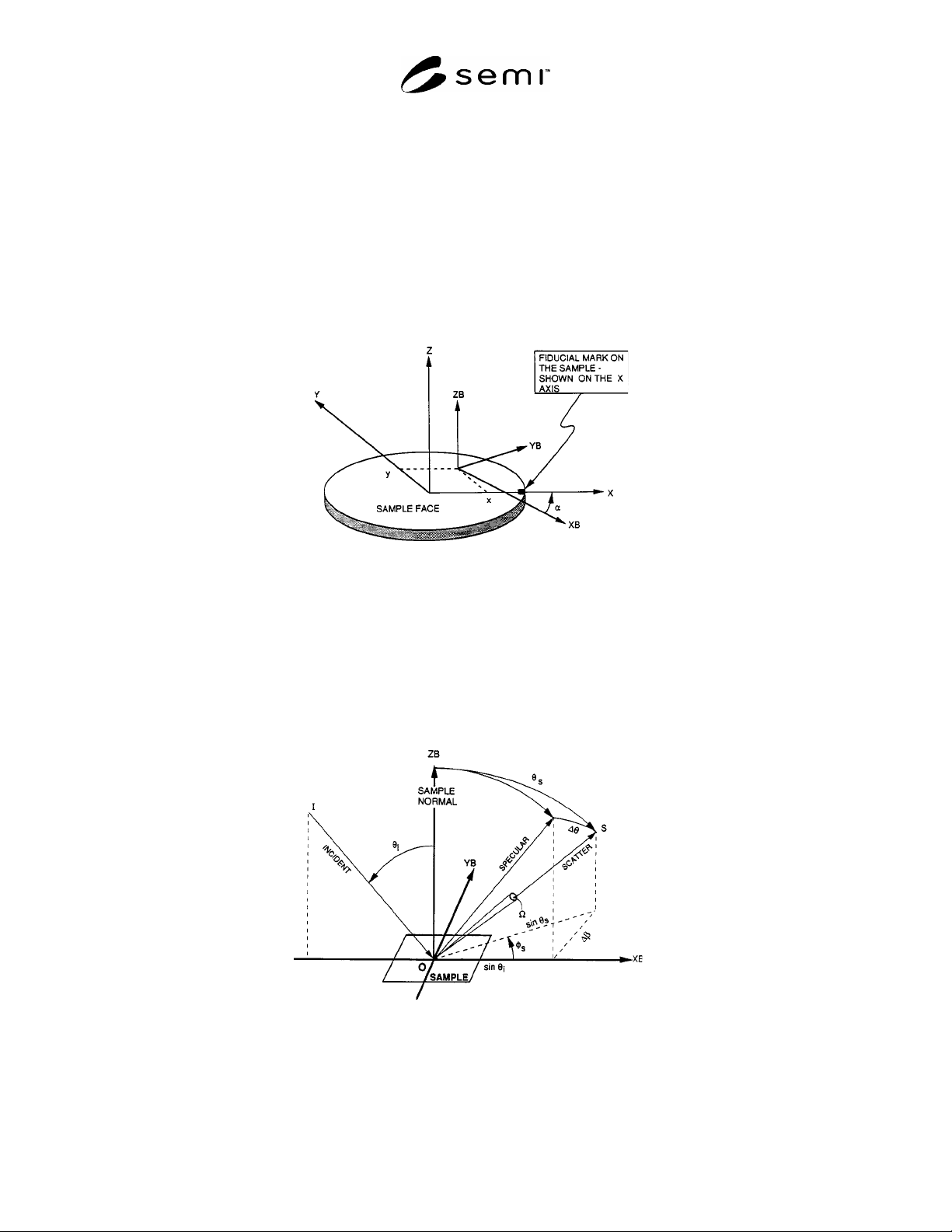
A1-1 Relationship between the Sample (X, Y, Z) and Beam (XB, YB, and ZB) Coordinate Systems
A1-1.1 The Z and ZB axes are always the local normal to the sample face. Locations on the sample face are
measured in the sample coordinate system. The incident and scatter directions are measured in the beam coordinate
system. If the sample fiducial mark is not an X axis mark, the intended value must be indicated on the sample (see
Figure A1-1).
NOTE 1: The X-Y zero position on the sample face is assumed to be the geometric center of the sample.
NOTE 2: The fiducial mark can be on the edge or back of the sample. For silicon wafers, the primary fiducial mark (flat or
notch) is on the circumference of the wafer at its intersection with the –y-axis.
Figure A1-1
Relationship Between Sample and Beam Coordinate Systems
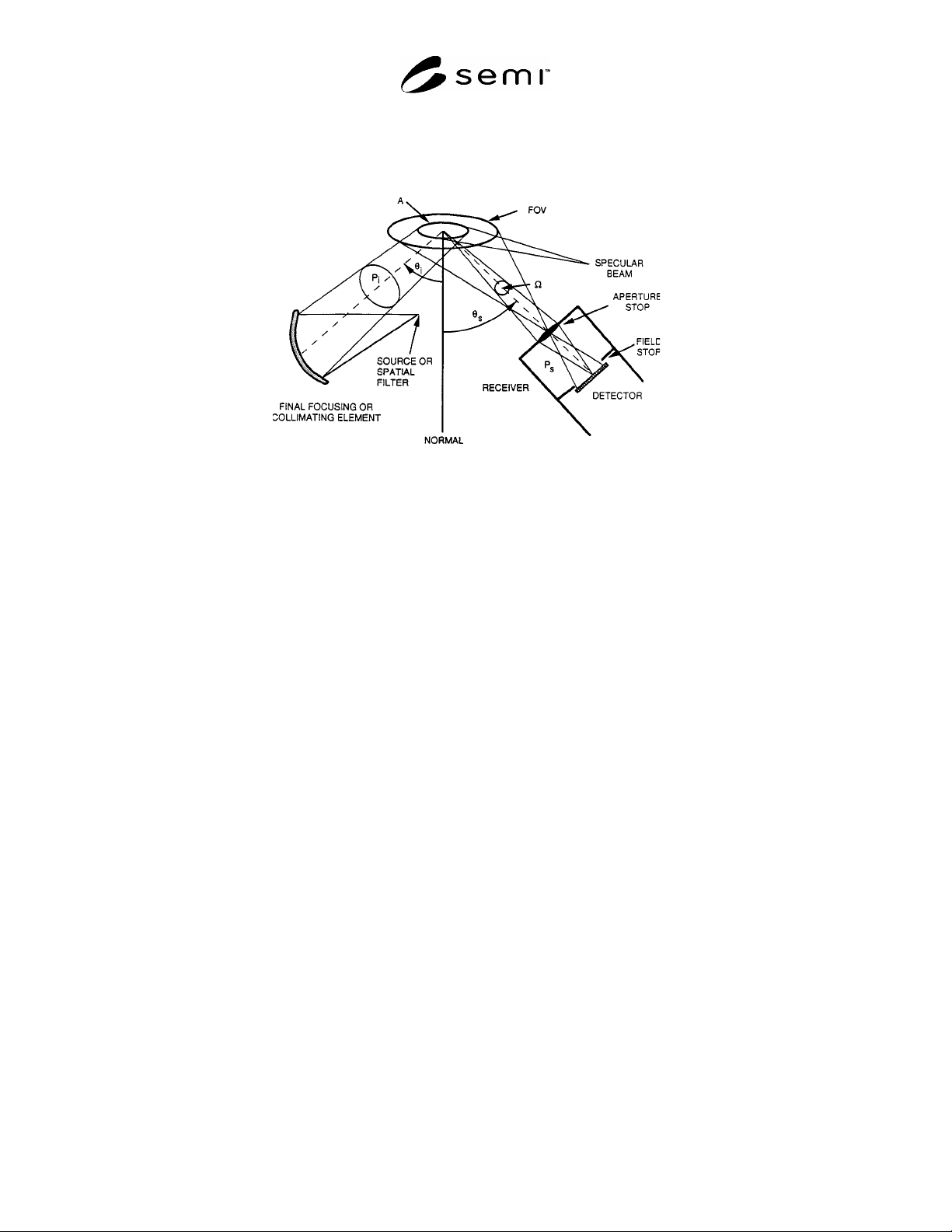
A1-2 Angle Conventions for the Incident and Scattered Light in the Beam Coordinate System
A1-2.1 The projection of the incident direction onto the sample face is the XB axis. Azimuth angles are measured
from the XB axis. The incident azimuth angle,
i
, is always 180° so
s
can be used directly in the common form of
the grating equation (see Figure A1-2).
NOTE: The plane of incidence (PLIN) is the I-O-ZB plane. The scatter plane is the S-O-ZB plane.
Figure A1-2
Angle Conventions
SEMI ME1392-0305 © SEMI 2003, 2005 11
A1-3 Receiver Geometry
A1-3.1 In many cases the field stop is set by the detector size; however, as the aperture stop approaches the field
stop the risk of seeing unwanted stray light increases. Other receiver geometries may be used. They all have
effective aperture and field stops and it is good operating practice to make them well defined.
NOTE: A = illuminated area with average E = P
i
/A, FOV = field of view that must include all area, A. The Aperture Stop limits
the size of , and the Field Stop limits the size of the FOV.
Figure A1-3
Receiver Geometry

SEMI ME1392-0305 © SEMI 2003, 2005 12
RELATED INFORMATION 1
ADDITIONAL DATA PRESENTATION
NOTICE: This related information is not an official part of SEMI ME1392 and is not intended to modify or
supercede the officiall standard. It was developed during the original approval of this standard by ASTM
Committee E12 in 1996. SEMI approval was by full letter ballot procedures with publication authorized by the NA
Regional Standards Committee on December 10, 2004. Determination of the suitability of the material is solely the
responsibility of the user.
R1-1
Presentation
R1-1.1 It is common practice to plot BRDF with respect to the angle from the specular beam,
. If scatter is
measured only in the PLIN,
=
s
i
. However, in the more general case for scatter out of the PLIN:
ssisi
cossinsincoscoscos
1
(R1-1)
R1-1.2 This is a useful angular reference for specular samples. However, when using this format, care must be
taken that
is not confused with
s
in the calculation of BRDF. This presentation format is normally used only
when
passes through zero, that is, when the scatter scan includes the specular beam.
R1-1.3 The terms “forward scatter” and “back scatter” refer to PLIN scatter directions for which
is respectively
positive or negative. Note that
continues to increase as a negative angle when passing the surface normal since
the sign of
s
switches in the above equation.
R1-2
Presentation
R1-2.1
=
o
, where
= sin
s
and
o
= sin
i
, is a method of expressing the angle between the specular and
scatter directions in direction cosine space along the surface for scatter in the PLIN. This is a very useful
normalization when scatter results only from surface microroughness, and the grating equation:
fn
is
sinsin (R1-2)
where:
= wavelength of the incident flux,
f = linear spatial frequency for the microroughness in the x or y direction, and
n = diffraction order.
This equation can be used to relate
s
to the frequency, f. Only the first order (n = 1) is significant for roughness
much less than the wavelength. BRDF can now be interpreted as the ability of each frequency to scatter light. If
BRDF is plotted against a
scale it may be independent of
i
and proportional to f. If the surface behaves in this
way the BRDF is “shift invariant.”
11
R1-2.2 In the general case for scatter out of the PLIN the following two dimensional grating equations apply:
xiss
fn
sinsincos (R1-3)
and
yss
fn
sinsin
(R1-4)
The definition of
must be expanded to include the projection of the scattered light in the X and Y directions:
ssisi
cossinsin2sinsin
222
(R1-5)
11 Harvey, James E., “Light Scattering Characteristics of Optical Surfaces,” Proceedings SPIE 107, 41 (1977)