semi合集-English.pdf - 第957页
SEMI E124-1103 © SEMI 2003 12 R1-1.8 Thus, if we set nor malized pro duction efficiency to have a value of ½ at this average cycle time , we get () () () ( ) {} () ( ) () 1 2 min , 1 normalizing exponent normalizing expo…

SEMI E124-1103 © SEMI 2003 11
R1-1.6 We can now see why the efficiency of
throughput rate and cycle time can both be measured by
the same metric (throughput-rate and cycle-time
efficiency). The following derivation also gives
alternative definitions for throughput-rate and cycle-
time efficiency for use when cycle time information is
not available (such as in resource-based simulations).
(
)
-
-
throughput rate and
cycle time efficiency
()
()
()
max ,
max ,
-
average WIP
theoretical
cycle time
bottleneck throughput rate
average cycle time
average
WIP
theoretical
cycle ti
best case cycle time
average cycle
me
bottleneck
throughput
rat
time
e
=
=
=
()
()()
()
()
1
max ,
1
min
average
WIP
average average
cycle time WIP
theoretical cycle time
bottleneck
average WIP
throughput rate
actual throughput rate
actual throughput rate
average WIP
theoretical cycle
=
=
()
()()
()( )
,
-
bottleneck
throughput rate
time
finished units out total time
average WIP theoretical cycle time
act
theoretical cycle time finished units out
ual throughput
total ti
rate
best case throughput rat
m
e
ea
=
=
=×
()()
as a fraction of
verage WIP
theoretical cycle time WIP
total time turnover
=×
(2)
R1-1.7 The production efficiency is normalized by the
power of the normalizing exponent so that a value of ½
for the normalized production efficiency indicates that
the factory is performing at the level of the threshold
case (which divides a well run factory from one badly
operated). This threshold case is also known as the
practical worst case, because it represents what the best
operating procedures can do in a maximally random
factory (see the Factory Physics book for more on this
case). In the threshold case,
()
(
)
(
)
1
average critical
WIP WIP
average
cycle time
bottleneck throughput rate
+−
= (3)
which results in the following production efficiency.
(
)
production
efficiency
(
)
(
)
()
()
()
()
-
-
max ,
max
throughput rate and WIP
cycle time efficiency efficiency
average
WIP
theoretical
cycle time
bottleneck
throughput
rate
WIP
efficiency
average cycle time
bo
theoretical
cycle time
=×
=×
×
=
()
()( )
()
()( )
{}
,
max ,
ttleneck
average
throughput
WIP
rate
average bottleneck
cycle time throughput rate
WIP efficiency
critical average
WIP WIP
×
×
=
()( )
{}
()( )
{}
min ,
max ,
average bottleneck
cycle throughput
time rate
critical average
WIP WIP
critical average
WIP WIP
×
×
()( )
{}
()()
()
min ,
1
critical average
WIP WIP
average critical
WIP WIP
bottleneck
throughput rate
=
+−
bottleneck
throughput
rate
×
()()
{}
()()
min ,
1
average critical
WIP WIP
average WIP critical WIP
=
+−
(4)

SEMI E124-1103 © SEMI 2003 12
R1-1.8 Thus, if we set normalized production
efficiency to have a value of ½ at this average cycle
time, we get
()
()
()()
{}
()()
()
1
2
min ,
1
normalizing
exponent
normalizing
exponent
normalized
production
efficiency
production
efficiency
average critical
WIP WIP
average critical
WIP WIP
=
=
=
+−
(5)
and, taking logarithms of both sides,
2
1
log
2
()()
{}
()()
()
()()
{}
()()
2
2
min ,
log
1
min ,
log
1
normalizing
exponent
average critical
WIP WIP
average critical
WIP WIP
average critical
WIP WIP
normalizing
exponent
average critical
WIP WIP
=
+−
=×
+−
(6)
so
()
()()
{}
()()
()()
()()
{}
()()
2
2
2
2
1
log
2
min ,
log
1
1
1
log
min ,
1
log
normalizing
exponent
average critical
WIP WIP
average critical
WIP WIP
average critical
WIP WIP
average critical
WIP WIP
average critical
WIP WIP
=
+−
−
=
+−
−
=
+
()()
{}
1
min ,
average critical
WIP WIP
−
(1)
which is the same as Equation (9) that was given in
Section 6 of the main body of this guide.
SEMI E124-1103 © SEMI 2003 13
RELATED INFORMATION 2
EXAMPLE APPLICATION
NOTICE: This related information is not an official part of SEMI E124 and was derived from an example
developed by the task force using this guide. This related information was approved for publication by full letter
ballot on April 11, 2003.
R2-1
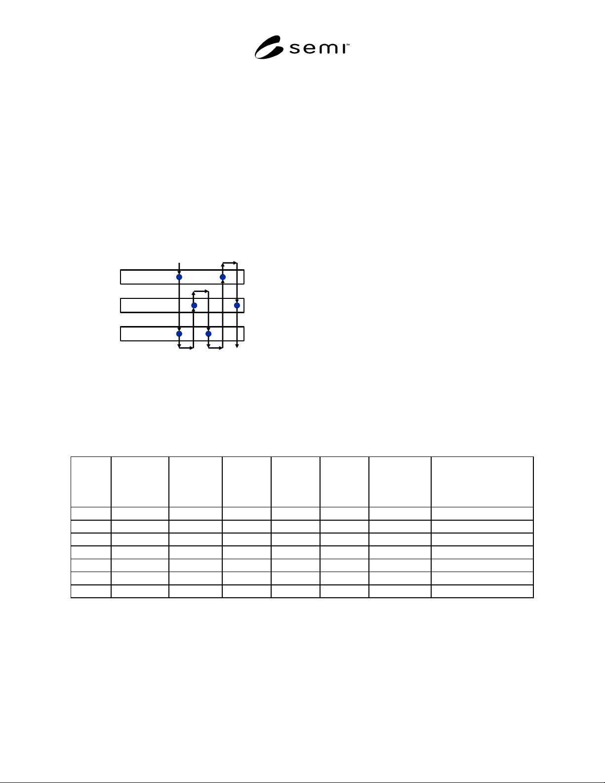
R2-1.1 As an example to show how the metrics in this
guide are applied, the diagram in Figure R2-1 shows the
process flow for a grossly simplified model of a wafer
fab (developed by Karl Kempf at Intel) that has only
five machines in three tool sets, one process flow with
six steps, and a single material handling vehicle (that
transports 25 wafers at a time).
Diffusion
Dry Etch
Lithography
Figure R2-1
MiniFab Process Flow
R2-1.2 The data for this model are shown in the first
few columns of Table R2-1 and Table R2-2. A
simulation gave the following additional run data:
total time = 9 years = 4,733,640 minutes
average cycle time = 1.8 days = 2,592 minutes
total units out = 39,420 lots = 985,500 wafers
finished units out = 938,571 wafers
scrapped units out = 46,929 wafers
good unit equivalents out = 891,642.1 wafers
R2-1.3 In the next-to-last column of Table R2-1, we
added together (for each step) all of the times (to load,
process batch, unload, and travel to next step) and
summed the results to get a theoretical cycle time of
812.4 minutes. In the last column of Table R2-1, we
computed the theoretical production time per unit for
each step. These values were then used in the last
column of Table R2-2 to compute the throughput rate
for each equipment set. The throughput rate for the
lithography equipment set (0.2182 wafers/minute) is the
bottleneck throughput rate, not because it is the
smallest throughput rate (it is), but because the
lithography equipment set has the highest average
operational efficiency. The remaining terms are
derived on the following pages.
Table R2-1 Process Data
Process
Step
Number
Equipment
Set
Name
Time to
Load
Batch,
minutes
Time to
Process
Batch,
minutes
Time to
Unload
Batch,
minutes
Time to
Travel to
Next Step,
minutes
theoretical
cycle time
(See Note 1),
minutes
theoretical production
time per unit
(See Note 2),
minutes/wafer
1 Diffusion 20 225 40 8 293 3.0
2 Dry Etch 15 30 15 4 64 1.2
3 Lithography 10 2.2 10 4 26.2 2.2
4 Dry Etch 15 50 15 8 88 2.0
5 Diffusion 20 255 40 4 319 3.4
6 Lithography 10 2.2 10 - 22.2 2.2
Sum - 90 564.4 130 28 812.4 -
NOTE 1: (theoretical cycle time) = (Time to Load Batch) + (Time to Process Batch) + (Time to Unload Batch) + (Time to Travel to Next Step)
NOTE 2: (theoretical production time per unit) = (Time to Process Batch)/(Process Batch Size)