semi合集-English.pdf - 第844页

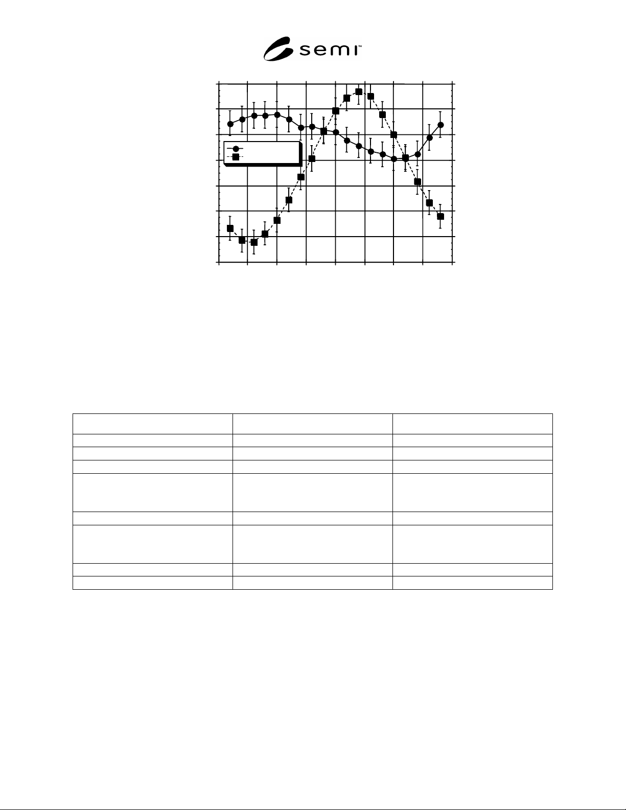
900 920 940 960 980 1000 1020 1040 -200 -150 -100 -50 0 50 100 150 200 Supplier A Supplier B Forward P ower (W) Reflection Coeffi cient Phase Angle (degrees) VSWR = 2 NOTE 1: The requested power was 1000 W. This plot sho…

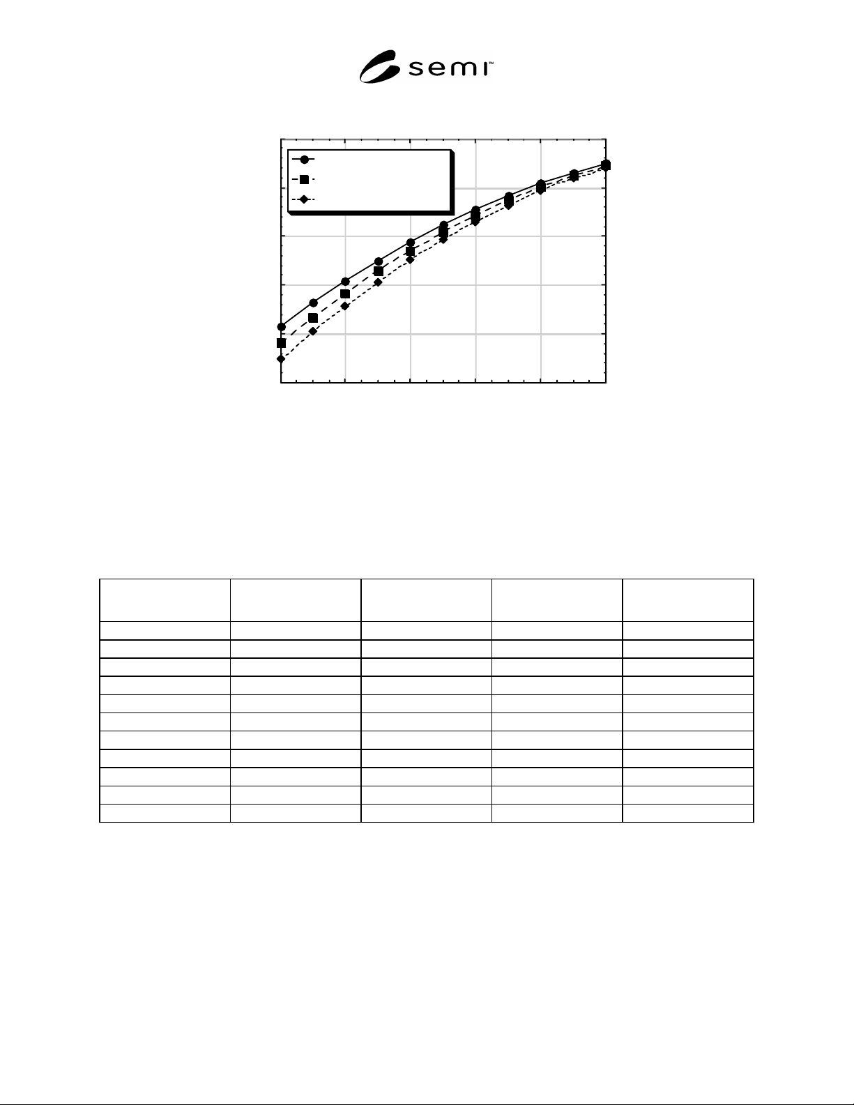
50.0

60.0

70.0

80.0

90.0

100.0

0246810

Tune = 3.0 volts

Tune = 5.0 volts

Tune = 7.0 volts

Power Efficiency (%)

Load Position (volts)

NOTE 1: The Tune Position is at the indicated fixed value for each set of data. For this example, the full-scale voltage for both

the Tune and Load Positions is 10 V (i.e., Tune = 3.0 V corresponds to 30% of full scale).

Figure 3

Example Plot of the Power Efficiency as a Function of the Load Position Tuning Element in the Matching

Network

Table 1 Example Data Table Showing the Matching Network Load Impedance and Power Efficiency as a

Function of the Positions of the Tuning Elements

Load

Position, volts

Tune

Position, volts

Real Load, ohms Reactive Load, ohms Power Efficiency, %

0 3 0.74 –31.75 61.51

1 3 0.91 –31.23 66.36

2 3 1.12 –30.64 70.86

3 3 1.38 –29.96 75.04

4 3 1.72 –29.18 78.88

5 3 2.15 –28.26 82.38

6 3 2.72 –27.17 85.56

7 3 3.50 –25.87 88.39

8 3 4.59 –24.31 90.90

9 3 6.18 –22.42 93.07

10 3 8.57 –20.15 94.91

NOTE 1: For this example, the full-scale voltage for both the Tune and Load Positions is 10 V (i.e., Tune = 3.0 V corresponds to 30% of full

scale). This example only shows data for a fixed Tune position of 3.0 volts. Data is also required at a Tune position of 0.0 V, 1.0 V, etc.

SEMI E113-1104 © SEMI 2001, 2004 9

900

920

940

960

980

1000

1020

1040

-200 -150 -100 -50 0 50 100 150 200

Supplier A

Supplier B

Forward Power (W)

Reflection Coefficient Phase Angle (degrees)

VSWR = 2

NOTE 1: The requested power was 1000 W. This plot shows a comparison of two different generators. The “Supplier A” data

(circles with solid curve) is within the required  1.5% variation from requested power (within the error bars), while the

“Supplier B” data (squares with dashed line) is not within the required  1.5% variation from requested power.

Figure 4

Example Data for the Forward Power as a Function of the Reflection Coefficient Phase Angle for a Nearly

Constant Value of VSWR/Reflection Coefficient magnitude (VSWR = 2)

Table 2 Example Data Table (Partial) Showing the Frequency Response of a Chuck Assembly

Test Frequency, MHz Refection Coefficient Magnitude Refection Coefficient. Phase, degrees

1.0 0.99973 –9.702

1.3365 0.99969 –12.95

1.673 0.99959 –16.18

41.097 0.9974 –180

135.2635 0.99488 25.94

135.6 0.99490 25.36

NOTE 1: The first column is the test frequency, the second column is the magnitude of the reflection coefficient, and the third column is the

phase angle of the reflection coefficient.

0.994

0.995

0.996

0.997

0.998

0.999

0 20 40 60 80 100 120 140

Refection Coefficient Magnitude

Frequency (MHz)

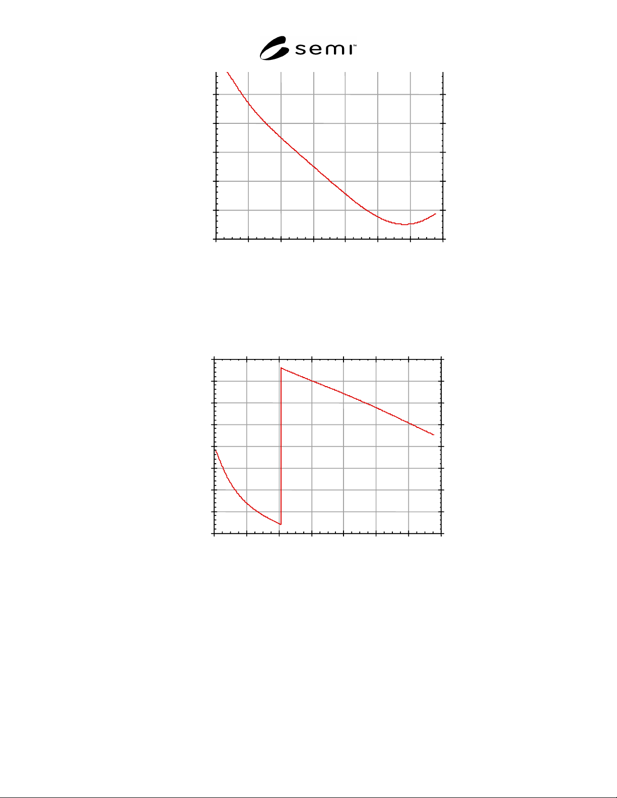
NOTE 1: This plot is the graphical form of the data shown in Table 2.

Figure 5

Example Data of the Magnitude of the Reflection Coefficient of the Chuck Assembly Plotted as a Function of

Frequency

-200

-150

-100

-50

100

150

200

0 20 40 60 80 100 120 140

Refection Coefficient Phase (degrees)

Frequency (MHz)

NOTE 1: This plot is the graphical form of the data shown in Table 2.

Figure 6

Example Data of the Phase Angle of the Reflection Coefficient of the Chuck Assembly Plotted as a Function

of Frequency