semi合集-English.pdf - 第7502页
SEMI MF1723-1104 © SEMI 2004 8 of zone lengths required to reach the flat portion of the axial concentration profile determines the length of ingot that must be grown to ac hieve an accurate carbon value. Figure 4 shows …
SEMI MF1723-1104 © SEMI 2004 7
be acceptable, choose sampling points for acceptor,
donor, and carbon sample wafers. Cut the sample
wafers at the proper points, then analyze for acceptor
and donor content by SEMI MF1389 and/or SEMI
MF1630, and for carbon by SEMI MF1391. Cut wafers
about 2-mm thick from the ingot for these analyses and
prepare the samples in accordance with the method
being used. Choose the ingot sampling plan
appropriate to the type of core being sampled in
accordance with the procedure in Sections 12.6.2 or
12.6.3 as appropriate.
12.6.2 Parallel Cores — For parallel cores (see
Section 10.2.1), single crystal ingot size is about 10 mm
diameter by about 200 mm in length. Select the
sampling points according to the individual segregation
coefficients for the specific impurities so these are
representative of more than 90% of the impurity
concentration as follows:
12.6.2.1 Segregation Effects — During the growth of
the crystal, crystallization from the melt, the impurity
concentration in the solid phase is different from that of
the liquid phase due to segregation.
1,2
The different
impurities have different segregation coefficients,
defined as:
l
s
C
C
K
0
(1)
where:
K
0
= equilibrium segregation coefficient,
C
s
= concentration of the impurity in the solid phase, in
atoms/cm
3
, and
C
l
= concentration of the impurity in the liquid phase, in
atoms/cm
3
.
12.6.2.2 Do not use the equilibrium segregation
coefficient for calculations since it is applicable only
for solidification at a negligibly slow growth rate. For
higher solidification rates, the impurity atoms are
rejected by the advancing melt at a greater rate than
they can diffuse into the melt. The impurity atoms
accumulate in the melt layer near the growth interface,
developing an impurity concentration gradient. The
concentration of this gradient depends on the growth
rate, fluid flow in the melt, and diffusion behavior of
the dopant. An effective segregation coefficient, K
eff
, is
described as:
)/exp()1(
00
0
DVKK
K
K
eff
(2)
where:
V = the growth rate, in cm/s,
= the diffusion layer thickness, in cm, and
D = the diffusion coefficient of the impurity in the
melt, in cm
2
/s.
12.6.2.3 In practice, measure a doping profile to
determine the concentrations of impurities along the
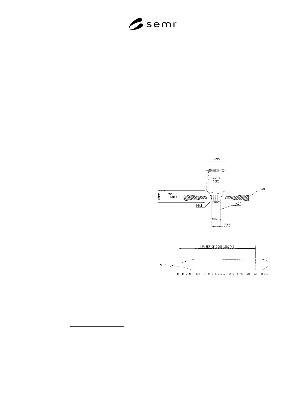
length of the ingot. The zone length, shown in Figure
3, is dependent on sample diameter, coil design, and
pull rate. After initial determination of the zone length,
re-measure it only after changes occur in the method
and apparatus. The doping profile, measured for each
impurity, determines where the ingot should be cut to
provide accurate impurity values. Sample points should
be chosen to be representative of more than 90% of the
impurity concentration. In Figure 3, the zone length is
measured at 15 mm. If the doping profile indicates that
the flat portion of the curve is at 12-zone lengths for an
impurity, take the sample at 12-zone lengths (12 × 15
mm = 180 mm) from the start of solidification on the
ingot.
Fi
g
ure 3
Zone Length Measurement and Ingot Sampling
Point
12.6.2.4 Ingot Profiling— For the type of float zone
furnace, coil design, pull rates, and ingot/core sample
diameter used, the effective segregation coefficient for
the impurities can vary. To calibrate the individual
zoner parameters and technique used, measure the
actual segregation coefficient profile. For example, to
determine the carbon profile, cut an ingot into wafers
along its length, and measure the carbon content in each
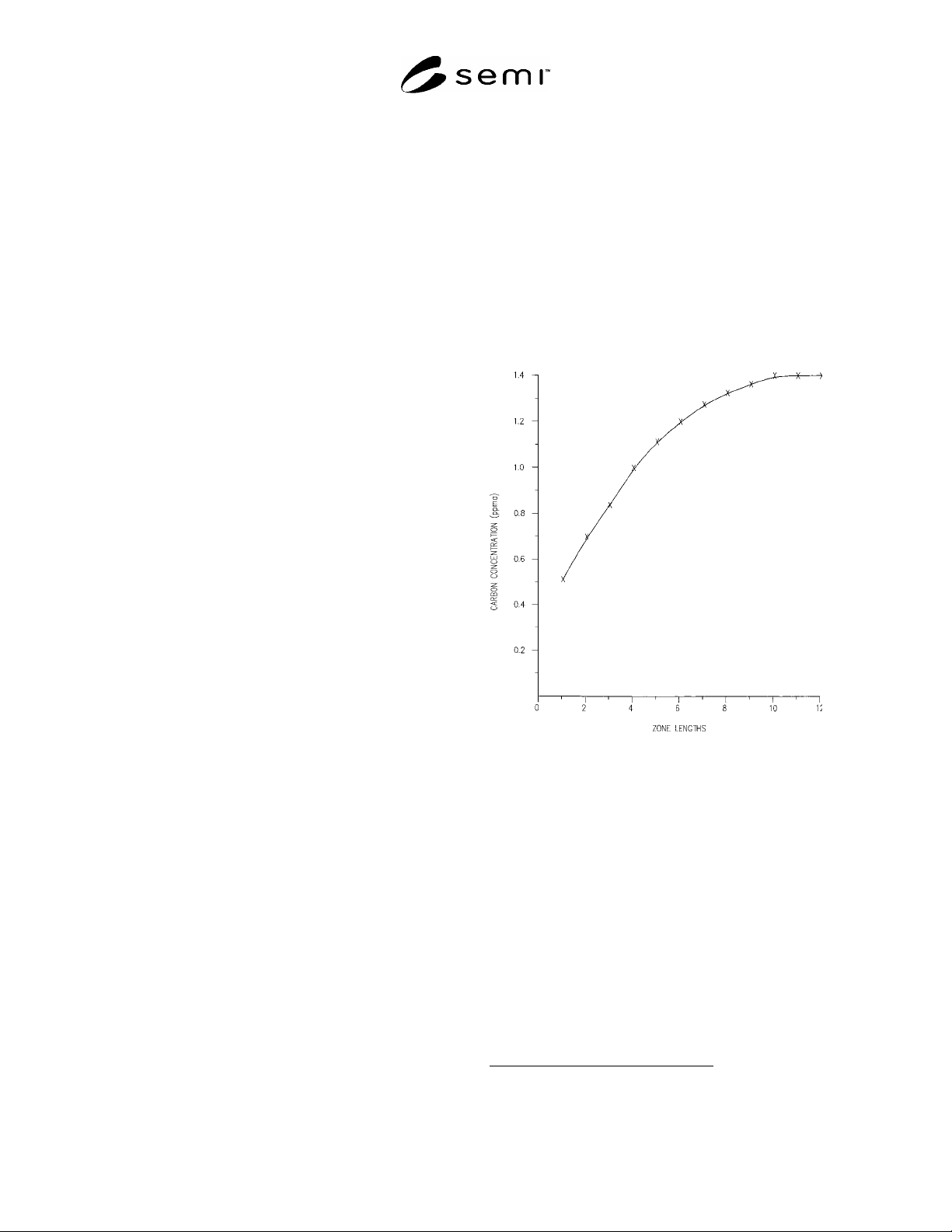
of the wafers. Then make a plot of carbon
concentration as a function of zone length. The number
SEMI MF1723-1104 © SEMI 2004 8
of zone lengths required to reach the flat portion of the
axial concentration profile determines the length of
ingot that must be grown to achieve an accurate carbon
value. Figure 4 shows an axial doping profile for
carbon where a 20-mm diameter sample core was zoned
to a 10-mm diameter ingot with a zone length of 15
mm. The effective segregation coefficient was 0.175.
In this case, growing the ingot to a zone length of 12
ensures that the maximum amount of carbon has been
incorporated into the ingot. Sampling the ingot for
carbon at a zone length of 12 gives reproducible carbon
values that accurately reflect the amount of carbon in
the polysilicon sample.
12.6.2.5 Slice Locations — Once the concentration
gradient for each element for the individual zoner
conditions is established, establish sampling rules for
each element. Boron, with a high segregation
coefficient, has a relatively flat profile. A wafer taken
from the ingot at 6 zone lengths has a value nearly
equal to that taken at 12 zone lengths. If one value is
significantly higher than the other, a contamination has
probably occurred, and the analysis should be repeated.
Phosphorus, with a smaller segregation coefficient, has
different values at the 6- and 12-zone length points.
The midpoint should have a value about 10 to 15%
lower than the end point. If not, contamination is
indicated and the analysis should be repeated. Carbon,
with a very small segregation coefficient, varies greatly
between the 6- and 12-zone length points. If not,
contamination is indicated and the analysis should be
repeated. Carbon value at the maximum ingot length
should be reported.
12.6.3 Perpendicular Cores — For perpendicular cores
(see Section 10.2.2), single crystal ingot size is about
14-mm diameter with a length determined by the poly
rod diameter, about 100 mm. For these ingots,
sampling for acceptor-donor content is different than
the carbon sampling, due to the small segregation
coefficient for carbon. Sampling points are selected
according to the following:
12.6.3.1 Resistivity Profile — Determine the
distribution of acceptor/donor impurities along the
length of the ingot by plotting a resistivity profile of the
ingot at 10-mm intervals, in accordance with SEMI
MF397. Also profile conductivity type, in accordance
with SEMI MF42, at 10-mm intervals. Due to the
segregation effects discussed in Section 12.6.2.1,
characteristic purity of the filament, and other
interferences discussed in Section 3, the resistivity
profile will differ between laboratories. A typical
resistivity/type profile is established after repeated runs
on control rods and production samples. Significant in
the resistivity profile indicates point contamination or
nonuniformity of the deposition layer.
12.6.3.2 Slice Locations — Establish sampling rules
for each element based on the resistivity/type profile.
The single crystal ingot length is correlated to the
polysilicon rod diameter; take a slice at the
representative midpoint between the filament and the
outer skin of the polysilicon rod. Analyze this wafer
for acceptor/donor values in accordance with SEMI
MF1389 or SEMI MF1630. For the cross section of a
polysilicon rod, these values represent the R/2 location.
If the resistivity/type profile has significant variation
from the standard profile, other locations may be
sampled to determine the distribution of each impurity.
Repeat the analysis for ingots with significant variation
suggesting point contamination.
Figure 4
Axial Doping Profile for Carbon
12.6.3.3 Carbon Analysis — Since accurate carbon
values can not be obtained on short ingot lengths,
perform the analysis on polysilicon sections that have
been annealed.
6
Take a second perpendicular
polysilicon core sample and anneal it at approximately
1360°C for 2 h. Take two 2-mm thick slices for the
carbon measurement in accordance with SEMI
MF1391. Take one sample from the point
representative of the midpoint of the growth layer and
the other sample at the point representative of the
filament location. If desired, sample other locations for
measurement of radial distribution.
6 Hwang, L. L., Bucci, J., McCormick, J. R., “Measurement of Car-
bon Concentration in Polysilicon Using FTIR,” J. Electrochem. Soc.
138, 576-581 (1991).
SEMI MF1723-1104 © SEMI 2004 9
13 Calculation
13.1 After measurement of the acceptor, donor, and
carbon impurities in the cut wafers, relate these values
to the levels in the polysilicon by making the following
calculations.
13.2 Parallel Cores — For sampling parallel cores (see
Section 10.2.1) in cases where the filament may be
doped or have a different composition than the
deposition layer, make the following calculation in
order to determine values for the total rod product:
t
LDftff
TRP
A
CAACA
C
..
)()(
(3)
where:
C
TRP
= total rod product concentration of impurity, in
p
pba for donor and acceptor, and in ppma fo
r
carbon,
A
f
= area of filament, in cm
2
,
C
f
= concentration of impurity in the filament, in
p
pba for donor and acceptor, and in ppma fo
r
carbon,
A
t
= area of polysilicon rod, in cm
2
, and
C
D.L.
= concentration of impurity in deposition layer,
in ppba for donor and acceptor, and in ppma
for carbon.
13.2.1 This calculation assumes that the deposition
layer is uniform across the diameter of the polysilicon
rod. Verify this assumption by taking sufficient core
samples to cover the entire deposition layer.
13.3
Perpendicular Cores — For sampling
perpendicular cores (see Section 10.2.2) where ingots
have been grown as in Section 12.6.3, make the
following calculation in order to determine values for
the total rod product.
13.3.1
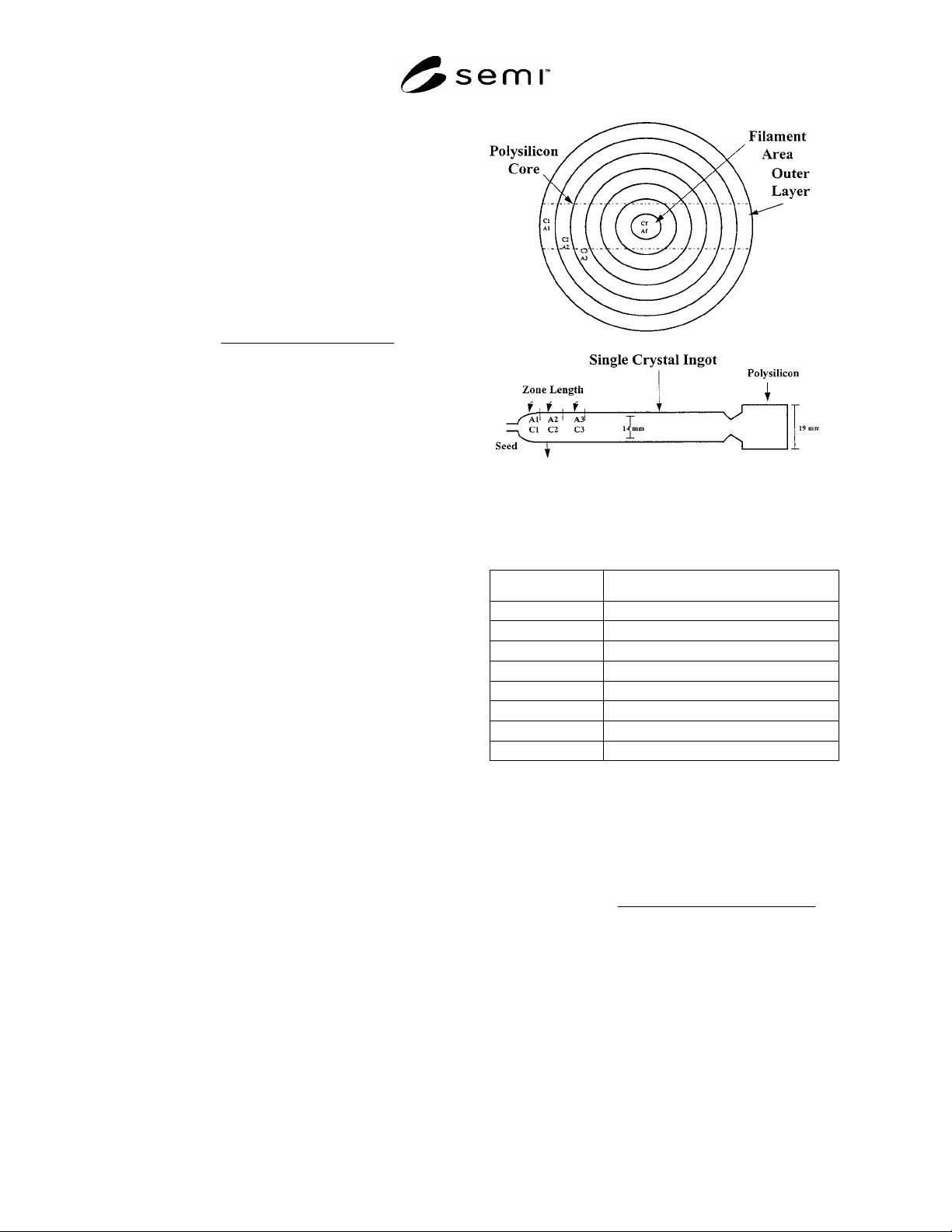
Correlate the single crystal ingot length to the
polysilicon rod cross section as shown in Figure 5. A
zone length is related to a cross section area. Boron,
with a large segregation coefficient, is assumed to have
an even distribution throughout the entire cross section.
Phosphorus, with a smaller segregation coefficient,
needs to be corrected for segregation factor for each
zone length across the cross section. Determine the
effective segregation coefficient for phosphorus, based
on repeated measurements of control rods for a specific
sample diameter, coil design, and pull rate.
NOTE 3: At one laboratory, segregation factors, based on an
effective segregation factor of 0.5, were calculated for the
zone lengths of Figure 5 as shown in Table 1.
Figure 5
Polisilicon Rod Cross Section
Table 1 Example of Phosphorus Segregation
Factors
Zone Length Segregation Factor
1 0.697
2 0.816
3 0.888
4 0.932
5 0.959
6 0.975
7 0.985
8 0.991
13.3.2 Use spectrophotometric values for boron
concentration (see SEMI MF1389 or SEMI MF1630)
directly in the following formula to calculate the total
boron concentration in the total rod product with no
correction for segregation:
A
f
2A1A
AfCf2C2A1C1A
C
VAC
K
K
(4)
where:
C
VAC
= volume averaged concentration,
A1,
A2,
Af
= corresponding area of poly rod cross section (see
Figure 5), and
C1,
C2,
Cf
= concentration of impurity at corresponding area,
corrected for segregation factor, where
necessary.