semi合集-English.pdf - 第7710页
SEMI T10-0701 © SEMI 2001 3 # of Pixel s Graysc ale Value Figure 2 Pixel Hi stogra m 5.1.18 qui et zone areas of space su r r o unding the machine-readable symbol. Quiet zone requirements may be found in application an…
SEMI T10-0701 © SEMI 2001 2
NOTE 1: Error correction techniques are described
extensively in AIMI Uniform Symbology Specification - Data
Matrix.
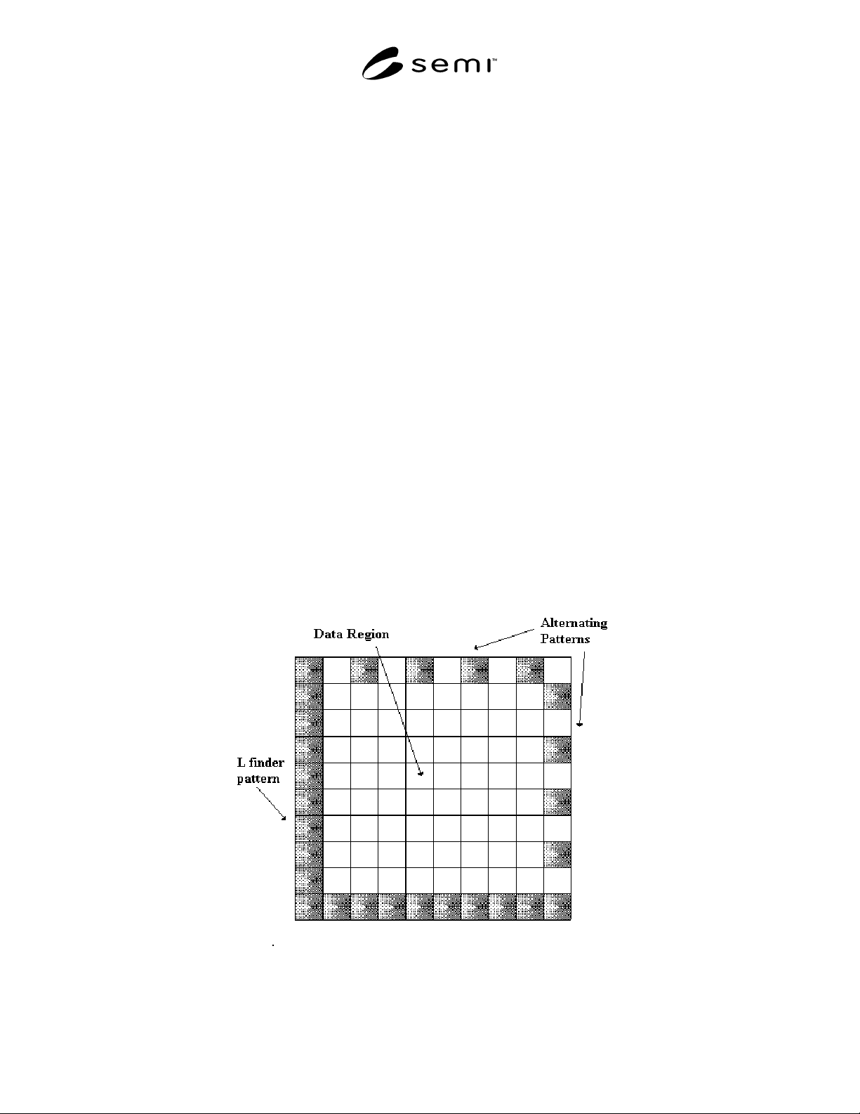
5.1.11 finder pattern, of a Data Matrix symbol a
perimeter to the data region. Two adjacent sides
contain marks in every cell: these are used primarily to
define physical size, orientation and symbol distortion.
This is often referred to as the L finder pattern. The
two opposite sides are made up of cells containing
marks in alternate cells (see Figure 1).
5.1.12 grayscale value
the assignment of a digital
value to a degree of light intensity. The shades of gray
are used by a computer to reconstruct an image. A
common scale is 256 shades of gray, with 0 being black
and 255 being white.
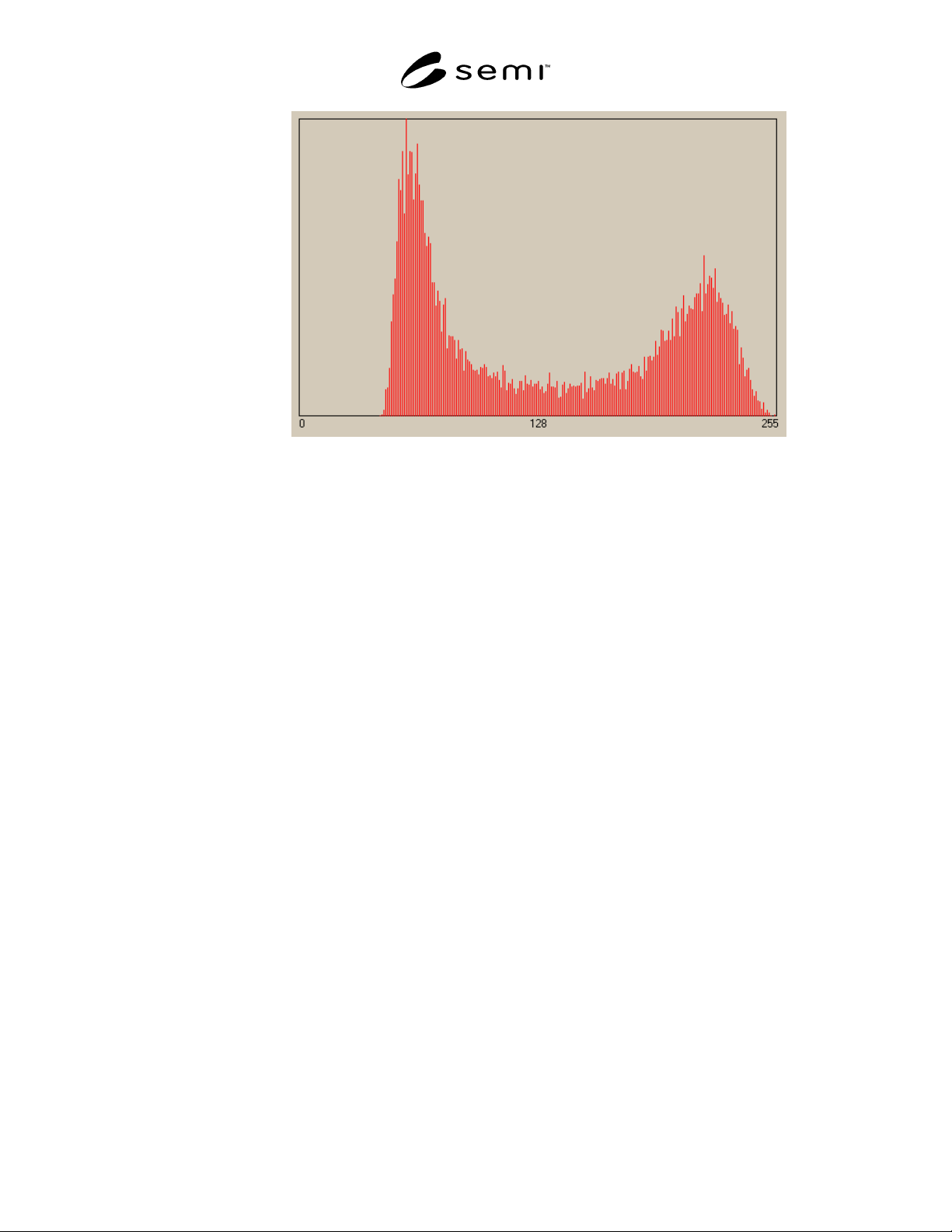
5.1.13 histogram a graphic representation of a
frequency distribution of pixel values within an area of
interest in a two-dimensional grayscale digital image.
The horizontal axis of the graph represents the range of
possible grayscale values in the image. The vertical
axis of the graph represents the frequency of occurrence
of each grayscale value in the area of interest (see
Figure 2).
5.1.14 image coordinates
location s in a two-
dimensional digital image are referenced by a two-
dimensional orthogonal coordinate system. The datum
for the coordinate system is in the upper-left corner of
the image. The horizontal axis or x-axis is located along
the top of the image, with increasing positive values
from left to right in the image. The vertical axis or y-
axis is located along the left side of the image, with
increasing positive values from top to bottom in the
image.
5.1.15 mark a cell or area of a Data Matrix symbol,
which has been marked, meaning the substrate has been
altered by the marking process so as to significantly
alter its contrast when imaged. Also can refer to an
entire Data Matrix symbol that has been applied in rows
and columns on a substrate by a marking process.
5.1.16 pixels picture elements. In a two-
dimensional digital image, pixels are individual
elements to which a grayscale value is associated. The
combination of grayscale values for each pixel and its
respective location in a two-dimensional plane form a
digital representation of a real scene.
5.1.17 pixel resolution
the precision in pixels at
which all measurements are performed. The maximum
pixel resolution shall be 1 pixel.
Figure 1
Data Matrix Symbol
SEMI T10-0701 © SEMI 20013
# of Pixels
Grayscale Value
Figure 2
Pixel Histogram
5.1.18 quiet zone areas of space surrounding the
machine-readable symbol. Quiet zone requirements
may be found in application and symbology
specifications. Sometimes called “Clear Area” or
“Margin.”
5.1.19 space
an unmarked cell or area of a Data
Matrix Symbol.
5.1.20 symbol a machine-readable pattern
comprised of a quiet zone, finder pattern, symbology
characters (which include special functions and error
detection and/ or correction characters) required by a
particular symbology.
5.1.21 symbol contrast the difference in grayscale
values between the marked and unmarked areas of a
Data Matrix symbol.
6 Summary of Method and R equirements
6.1 Test Image
6.1.1 A test image of the mark shall be obtained in a
configuration that mimics the typical reading
configuration for that mark, at substantially the same
resolution, illumination, optical focus, image exposure,
gain or other image signal preprocessing settings that
are used during reading. Individual applications may
dictate a specific wavelength or color temperature and
spatial construction of illumination, image resolution,
optical focus, image exposure, etc. The mark/reader
configuration shall be consistent to the extent that
repeatable results can be obtained from a single sample
over many instances of one mark/reader configuration.
6.1.2 The intent of the assessment p rocedure is to
regard a test image from the actual mark/reader
configuration as the source for all assessment.
Therefore, the assessment criteria and the algorithms
used to carry out each assessment should be resident in
the actual reading system or equivalent that is used to
read the mark. If a separate assessment or verification
system, which has different illumination characteristics,
resolution, etc., is used, uncorrelated results may occur.
6.2 Edge Detection Method
6.2.1 Many of the assessment proce dures depend
significantly on the type of edge detection method that
is employed to locate edges in the test image which
define the bounds of the entire Data Matrix symbol as
well as individual cells within the matrix. The edge
detection method used should be consistent throughout
the assessment process.
SEMI T10-0701 © SEMI 2001 4
7 Procedure
7.1 Location and Orientation of the Data Matrix
Symbol
7.1.1 Data Matrix Location Descrip tors
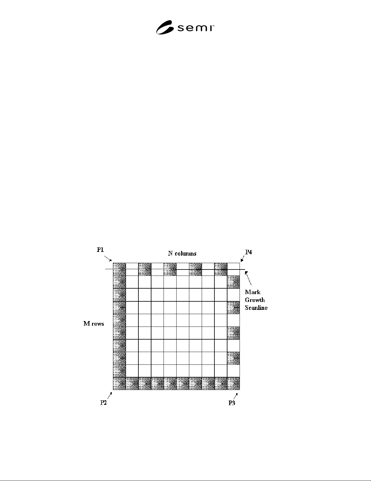
7.1.1.1 The implementation of the symbol quality
assessment depends on knowledge of the location and
orientation of the Data Matrix symbol in the image,
which consists of the 4 image coordinate values of the
matrix corner points, P1, P2, P3, and P4 (see Figure 3).
In addition, the number of rows M and the number of
columns N in the Data Matrix symbol is also required
(see Figure 3). Determine the image coordinate values
and the number of rows and columns using a pre-
processing decoding procedure resident in the reading
system. Should this process either fail or not be
available, determine these values by inspection of the
test image. Report the coordinate values of each matrix
corner point and the number of rows and columns.
7.1.2 The Data Matrix Grid
7.1.2.1 Based on the location of the 4 matrix corner
points and the number of rows and columns in the
matrix establish a geometrical 2 dimensional matrix
grid. Establish line segment P1P2 using points P1 and
P2, line segment P2P3 using P2 and P3, line segment
P3P4 using P3 and P4, and finally line segment P1P4,
using P4 and P1. Divide the number of rows M into the
P1P2 line segment, producing M equally sized line
segments. Divide the number of rows M into the P3P4
line segment producing a similar result. Divide the
number of columns N into P1P4 line segment,
producing N equal sized line segments. Divide the
number of columns N into the P2P3 line segment,
producing a similar result. Connect the corresponding
new line segment endpoints between P1P2 and P3P4.
Connect the corresponding new line segment endpoints
between P1P4 and P2P3. This results in a 2
dimensional matrix grid similar to that shown in Figure
3. This grid is generally quadrilateral in shape,
practically rectangular and ideally square.
7.1.3 Data Matrix Cell Center Point s
7.1.3.1 Determine the ideal geometric al center points
in each matrix cell in the following manner. Establish a
new set of points at the bisection of each row and
column line segment used to form the matrix grid.
Form line segments between each corresponding row
bisection point in P1P2 and P3P4. Do the same for the
column bisection points in P1P4 and P2P3. The
intersection points between this new set of lines in each
matrix cell is the ideal geometrical matrix cell center
point (see Figure 4).
Figure 3
Data Matrix Corner Points and Mark Growth Scanline