semi合集-English.pdf - 第3951页
SEMI F38-1104 © SEMI 1999, 2004 3 7.2.1 An exampl e of the appa ratus is shown in F igure 1. The input particle concentration is measured by CNC-B, while the output pa rticle concentration is measured by CNC-A. The press…
SEMI F38-1104 © SEMI 1999, 2004 2
a background level as specified in Section 7.1.2.
6.3 Test Environment — Particle challenge testing does
not require a clean area. Testing in a Class 100 area is
recommended but not required. Refer to Section 6.7 for
installation precautions.
6.4 Configuration for Efficiency Test — One example
of the configuration is shown in Figure 1. The setup
shown in Figure 1 is intended only as a guideline. This
system consists of:
an aerosol generation system,
aerosol concentration detectors,
an air flow measuring system,
a filter pressure drop sensor, and
the test filters.
6.5 Test Flow Rate — Maximum manufacturer’s rated
flow rate.
6.6 Challenge Particle Sizes — Experimentation of
various media (e.g., metallic, ceramic, and polymeric)
have resulted in most penetrating particle sizes ranging
from 0.05–0.11 micron.
1
2
3
4
6.6.1 Several monodispersed particle challenge tests
shall be done over a range of particle sizes so that
testing at the most penetrating particle size is
performed. An electrostatic classifier must be used to
produce a monodispersed challenge.
6.6.2 Due to the effects of particle loading in relation
to filtration efficiency, a clean filter should be used for
each particle size challenge. The differential pressure
across the test filter should be continuously monitored
to eliminate the possibility of particle loading. The
following particle increments are a guideline. Smaller
increments are achievable and are desirable.
6.6.2.1 Challenge Particle Size In Microns:
1 Rubow, K.L., C.B. Davis (1991) "Particle Penetration
Characteristics of Porous Metal Filter Media for High Purity Gas
Filtration", Proceedings of Institute of Environmental Sciences
Annual Technical Meeting
2 Rubow, K.L., and Liu, B.Y.H., Evaluation of Ultra-High Efficiency
Membrane Filters, Proceedings of the 30th Annual Technical
Meeting, Institute of Environmental Sciences, 1984.
3 Rubow, K.L., Liu, B.Y.H., and Grant, D.C., Characteristics of
Ultra-High Efficiency Membrane Filters in Gas Applications; Journal
of Environmental Sciences, May/June, 1988.
4 B. Gotlinsky, P. Conner, D. Capitanio, L. Johnson, and S. Tousi,
Testing of All-Metal Filters for High Purity Semiconductor Process
Gases, Proceedings of the 37th Annual Technical Meeting, Institute
of Environmentak Sciences, 1991.
0.05
0.07
0.10
6.7 Sample Installation — Reasonable precautions
shall be taken when installing the test filter to avoid
particle contamination of the system from ambient.
These precautions may include, but are not limited to:
installation in a Class 100 laminar flow area,
installation in a purged glove bag or other controlled
ambient enclosure, use of a purge flow downstream of
the sample point so that all parts of the system are
under purge, isolation, or termination of the CNC
sample flow, and isolation of the isokinetic sampler
exhaust from ambient.
6.8 Customary practices shall be employed for the
design of the sampling system. This includes any
specialized equipment or procedures recommended by
the CNC manufacturer. Every effort should be taken to
minimize differences in the particle concentrations of
the sampling volume relative to the actual test volume.
Care should be taken to provide an adequate exhaust
length so that back diffusion of particles does not affect
background at 2 times the sampling flow rate. This
length will depend upon the particle concentration in
the ambient environment and on other factors.
6.9 Test Particle — Solid non-volatile particles.
Sodium chloride is recommended, but other particles
could be used such as polystyrene latex beads (PSL) if
sufficiently high concentrations can be generated.
7 Procedure
7.1 Static Background Test
7.1.1 Purge the system at a high velocity flush of 100
slm or the maximum flow rate that the system
components will allow.
7.1.2 Purge the system at test flow rate (Section 6.5).
Measure the particle concentration with clean gas to
determine the background concentration. The
background count is established when the counter has
sampled a minimum of 3 scf (85 sl), and the arithmetic
average during the last 3 scf (85 sl) of gas sampled is
<2 particles/scf (<0.07 particles/sl). The sample
interval shall be 1 minute in duration. Ensure that the
background counts are stable or decreasing. If
background cannot be achieved after 6 scf (170 sl) have
been sampled, there may be a problem with the counter
or test apparatus. Past experience has shown this to be
an adequate volume of gas to give a satisfactory low
level background particle counts.
7.2 Penetration Test
SEMI F38-1104 © SEMI 1999, 2004 3
7.2.1 An example of the apparatus is shown in Figure
1. The input particle concentration is measured by
CNC-B, while the output particle concentration is
measured by CNC-A. The pressure and flow rates in
both legs should be carefully balanced (by maintaining
an identical differential pressure in both legs) to insure
that the challenge level is the same.
7.2.2 Set the first and subsequent challenge particle
sizes per Section 6.6.
7.2.3 Particle challenge concentrations should be set to
the maximum output of the electrostatic classifier for
each of the particle size tests (Section 6.6). This will
determine the test volume and the duration of the test.
Generally this requires generating a polydispersed
aerosol having a mean size close to the desired
monodispersed aerosol size. Any difference between
the flow rate exiting the electrostatic classifier and the
test flow rate specified in Section 6.5 will be made up
by dilution gas as shown in Figure 1.
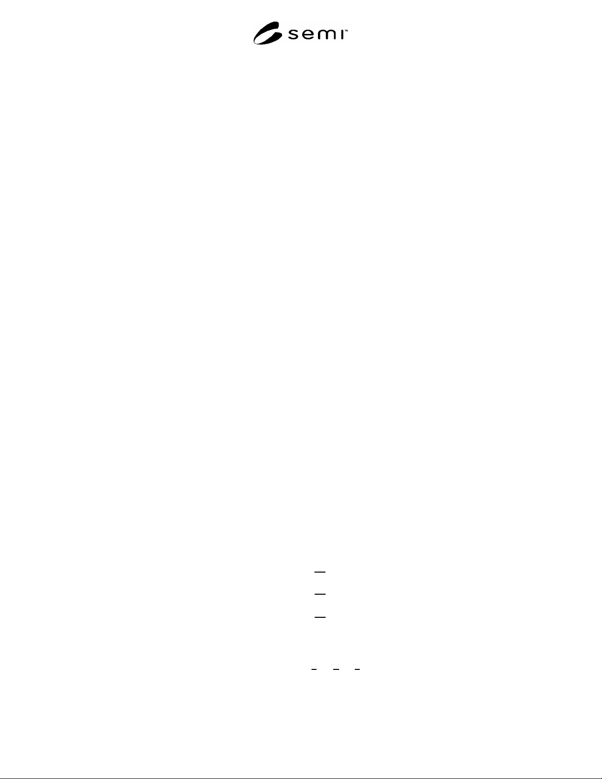
7.2.4 The total particle challenge must be limited to
1 10
9
particles per liter of filter rated flow in slm.
This is done to limit the effects of a particle cake build-
up which would enhance the efficiency of the test filter.
The test should be concluded upon exposure to 1 10
9
particles per liter of rated flow or after 10 downstream
counts are observed, whichever occurs first.
7.2.4.1 As an example, a 10 liter per minute filter
would be challenged in one minute with (10 slm) (1
minute) (1 10
9
particles/liter) or 1 10
10
particles.
If the challenge concentration is 1 10
8
particles per
liter and the flow rate is 10 slm, then the test would
need to last 10 minutes or when 10 downstream
particles were observed.
7.2.4.2 The sample interval shall be 1 minute in
duration. The sample interval in the penetration test is
equivalent to the sample interval in the system
background test (Section 7.1.2).
7.2.5 Measure the input and output particle
concentration.
7.2.6 Calculate the ratio of output to input particle
concentration.
8 Reporting of Test Results
8.1 Raw data shall be reported for each test in the
format of a table, including the number of sample
intervals, the sampling volume of each interval, the
sampling time of each interval, and the total number of
particles registered in each interval. In addition, the
relevant parameters for each test described in Sections
8.2 and 8.3 should be identified.
8.2 Static Background Test — Identify the period of
time required to obtain 45 consecutive sampling
intervals without a particle being detected for the spool
piece and test filter.
8.3 Penetration Test — Identify the input
concentration, the output concentration, the ratio of
output to input concentration (fractional penetration),
and the challenge particle size. The most penetrating
particle size is the challenge particle at the largest
fractional penetration. Care must be taken to distinguish
between true penetration and system background counts
(see Section 8.5) as measured in Section 7.1.2.
8.4 Efficiency Class
8.4.1 If no penetration is observed then report the POU
Gas Filter passed a X LRV efficiency test, where X =
the maximum detectable efficiency for the test (as
defined in Section 2.2). No penetration is defined as
when the filter output is not statistically different from
the system background (as defined in Section 8.5).
8.4.2 If penetration is observed , then report that the
POU Gas Filter failed a X LRV efficiency test, where X
is the maximum detectable efficiency for the test (as
defined in Section 2.2). Penetration is defined as when
the filter output is statistically different from the system
background (as defined in Section 8.5).
8.4.2.1 The LRV defines the number of nines in the
efficiency.
8.4.2.2 Example: A filter with a fractional penetration
of 0.00001 has a LRV of 5 and an efficiency of
99.999%
8.5 Data Reduction
8.5.1 The statistical analysis is based on the
assumption that the particles generated are randomly
distributed and are statistically independent of each
other. The background counts are independent of the
particle performance of the component. The particle
counts observed from the test include the counts from
the component and the background count.
Let:
X
B
= average background particle count
X
t
= average total particle count from test
X
c
= average particle count generated by the test
component
Therefore,
X
t
X
c
X
B
8.5.2 A statistical analysis of the data is performed to
SEMI F38-1104 © SEMI 1999, 2004 4
determine the mean, standard deviation, and the
standard error for each particle size range.
8.5.3 The sample mean, X, or average of the data for
each state is given by:
X
X
i
n
i 1
n
where X
i
is the observed counts for the state and n is the number
of samples.
8.5.4 The sample standard deviation is a measure of
the variability of the data about the mean. The standard
deviation, s, for each state is expressed as:
s
(Xi X
)
2
i1
n
n 1
8.5.5 The standard error, Se or standard deviation of
the sampling distribution of the mean for each state is
given below:
Se
s
n
8.5.6 The average particle count for the total number of
particles generated, or the sample mean, is an
estimation of the population mean. For a 95%
confidence level, the population mean, µ
p
, will be
within two standard errors of the sample mean, or:
p
X 2 Se
8.5.7 In order to determine if there is statistical
evidence of the component having an effect on the
observed particle count, a test must be conducted to see
if the actual difference between the average background
count, X
B
, and the average test count, X
t
, exceeds two
standard errors in a distribution of differences between
means. The average particle count generated by the test
component, X
c
, is given by:
X
c
X
t
X
B
8.5.8 The standard error in a distribution of differences
between means is expressed as:
S
ec
S
et
2
S
eB
2
8.5.9 The 95% confidence interval of the test
component itself is then determined by:
X
c 2 S
ec
8.5.10 If this confidence interval includes 0, then this
implies that there is not strong statistical evidence of
the component having an effect on the observed particle
count. If this interval does not include 0, then this
implies there is strong statistical evidence that the
component does have an effect on the observed particle
count.
8.5.11 Present in tabular form the average particle
count and the associated 95% confidence limits (as
calculated in Section 8.5.9) for each test state. In
addition, present the background test data separately as
a distinct element.
8.5.12 Calculation of the Efficiency Class
8.5.12.1 The efficiency class shall be calculated in
such a fashion that that:
LRV = Log [Input Concentration / X
B
+ 2S
eB
].