semi合集-English.pdf - 第5172页
SEMI M32-0998 © SEMI 1998, 2004 11 0 5 0 100 8 10 13 15 18 20 23 26 28 Figure A4-4 Error at 2 Sigma A4-3.7 The error when the speci fication is 2 sigma from the mean, shown in Figure A4-4 as the area between the vertical…
SEMI M32-0998 © SEMI 1998, 2004 10
A4-3.2 No control method can hold a process perfectly
still. Even the best real-time control methods can allow
a process to drift as much as ± 1.5 sigma. For this
reason, a 6-sigma design was defined as 4.5 sigma to
the nearest tolerance.
A4-3.3 Sampling issues are a major concern. Many
kinds of variation can be quantified by rigorously
studying the appropriate samplings (within batch
samples for batch-to-batch variation, monthly samples
for month-to-month variation, etc.). However, there are
practical limits on how many kinds of variation can be
continuously monitored. There is a large amount of
work involved, and there are hundreds of potential
sources of variation. Resource restrictions regularly
force suppliers to concentrate on the known key
variables and leave the rest as error in the system (at
least for now). As sample periods get longer, there is
more statistical sensitivity, but also more probability
that the drift will be confounded with user-driven
process improvements. For example, month-to-month
random drift is hard to quantify because production
processes are often improved before many months of
data can be observed. Measurement error is another
main contributor which further complicates the other
sensitivity issues. These factors all combine to allow a
certain amount of undetectable process drift. This
process drift needs to be considered when defining the
specification approach.
A4-3.4 These variations cannot be detected because of
statistical sensitivity limitations. Table A4-1 shows the
sample sizes needed to detect different levels of process
shift. Delta will be defined as the number of sigma of
undetectable mean drift. For simplicity, a one-way shift
is shown, but in most practical cases, the shift could go
plus or minus. Using the old standard of 5% supplier
risk and 10% user risk, 72 samples are needed to detect
a delta of 0.25 sigma. This example (0.25 sigma of
mean drift) has been used throughout this document.
Since most of the discussion will relate to process drift,
the terms “drift” and “shift” will be used
interchangeably. Clearly, 72 is too large a sampling for
most real-time control systems, but it is still an
understatement of the problem. Most users currently
expect their risk to be much smaller than 10%. The last
row shows that the sample size would need to be 311 to
reach 0.1% user and supplier risks. It is generally
agreed that 0.1% (i.e., 1000 ppm) is the lowest level
that is feasible using standard probability theory. For
lower levels, it is necessary to move farther out on the
distribution tails where it is necessary to rely on more
than just stndard sampling probabilities.
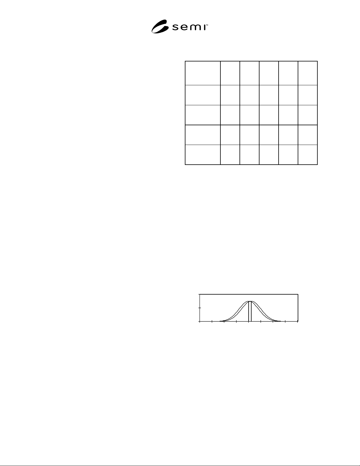
Table A4-1 Sampling Requirements
(a = supplier risk, b = user risk)
Detectable
Mean Shift
(in Sigma)
0.125 0.25 0.50 0.75 1.0
Min N
a = 20%
b = 20%
92 24 7 4 4
Min N
a = 5%
b = 10%
280 72 20 10 7
Min N
a = 1%
b = 1%
696 177 47 23 15
Min N
a = 0.1%
b = 0.1%
1228 311 82 40 25
A4-3.5 Figures A4-3, A4-4, and A4-5 show the error
generated by 0.25 sigma of undetectable mean drift.
Again, the number of sigma of undetectable mean drift
will be defined as delta. Notice how the error grows as
the point of interest moves toward the center of the
distribution. At the four sigma point (out on the tail)
there is very little error, so suppliers can be generous
with internal buffer specifications to protect the user.
This is not as feasible in the center of the distribution
because there is so much material at stake. A percentile
specification in the center of the process shown would
have about 1000 times more undetected, out-of-spec
product than a specification at the 4 sigma point. Since
the shift could go either way, this could also be 1000
times more material that was rejected and should not
have been.
0
50
100
8 1013151820232628
Figure A4-3
Error at 0 Sigma
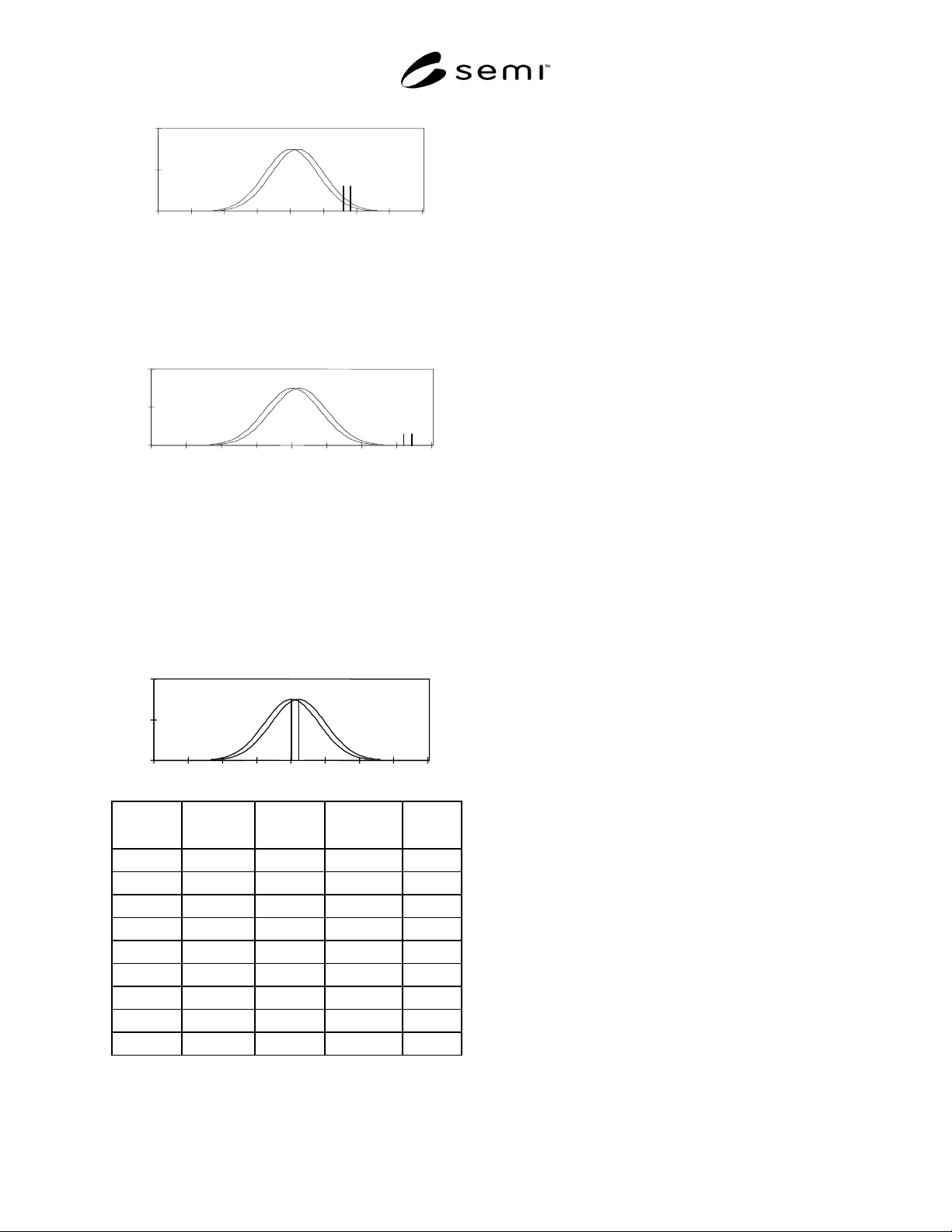
A4-3.6 The left curve in Figure A4-3 shows a
distribution with an expected mean of 18. The right
curve shows the same distribution with an undetectable
drift of 0.25 sigma. If a specification limit is placed at
18, then 50% of the material is below the specification
for the nominal distribution. However, only 40.13% is
below the specification for the distribution that has
drifted. The error, shown by the area between the
vertical lines and below the right curve, is 9.87% or
98,700 ppm.
SEMI M32-0998 © SEMI 1998, 2004 11
0
5
0
100
8
10
13
15
18
20
23
26 28
Figure A4-4
Error at 2 Sigma
A4-3.7 The error when the specification is 2 sigma
from the mean, shown in Figure A4-4 as the area
between the vertical lines and below the right curve, is
1.73% or 17,300 ppm.
0
50
100
8
10
13
15
18
20
23
26 28
Figure A4-5
Error at 4 Sigma
A4-3.8 The error when the specification is 4 sigma
from the mean, shown in Figure A4-5 as the area
between the vertical lines and below the right curve
(but indistinguishable), is 0.01% or 100 ppm.
A4-3.9 Figure A4-4 further quantifies this error.
Percent-less-than calculations are shown for each curve
at increments of 1 sigma from the mean. The starting
mean is 18, and the sigma is 2.
0
50
100
8
10
13
15
18
20
23
26 28
Value
Value
Description
Left
Curve %
Right
Curve %
Error
%
10 - 4 s 0.01 0.00 0.01
12 - 3 s 0.13 0.06 0.07
14 - 2 s 2.28 1.22 1.06
16 - 1 s 15.87 10.56 5.31
18 mean 50.00 40.13 9.87
20 + 1 s 84.13 77.34 6.79
22 + 2 s 97.72 95.99 1.73
24 + 3 s 99.87 99.70 0.17
26 + 4 s 100.00 99.99 0.01
Figure A4-6
Percentage Error
A4-3.10 Please note that this is a very conservative
example. The delta and the resulting error can get much
larger.
A4-3.11 A major concern is what to do when the
specification is not met. Users would certainly not want
suppliers to reject material in the center of the
distribution. Alternatives are to (1) reject the whole
shipment, (2) reject nearby lots, (3) mix and match lots,
or (4) translate the percentage hypothetically lost in the
center back out to the tail in order to reject the worst
material. The first two alternatives are really more like
penalties and would lead to unnecessary loss of good
material. The third is the worst form of inspecting in
quality. It is generally agreed that this is the main thing
to avoid. Translating the error back to the tail is
possible but not necessarily a good approach. This
would involve translating a reject percentage with a
large potential error back out to a region that would
have had a very small error. A multiple percentile
specification can also be quite difficult in a production
environment. Each of the percentile criteria must be
evaluated to determine which one requires the highest
reject rate. That reject rate must then be translated back
to the tail, and 100% sample data must be used to
determine which actual pieces to reject. If the statistical
distribution is defined, one specification would give the
same amount of information with much less work. If
only one criterion is used, and it is well out on the tail
(hopefully in the ppm range) then this method is very
similar to a statistical specification.
A4-3.12 A commonly stated goal of multiple percentile
specifications is to focus on centering rather than
distribution tails. All of the discussion in Section A4-
2.2 concerning centering is equally applicable here.
Multiple percentile specifications are more likely to
cause inspected-in quality which detracts from process
control based centering.
A4-3.13 Ease of use is another stated goal, but for all
of the reasons stated above, this method is one of the
most difficult to use. Statistical calculations can be
done in milliseconds while the potential of large
samplings, raw data manipulation, and duplicate effort
associated with multiple distributional percentile
specifications create much more work. Characterizing
with percentiles is an alternative for processes that have
not yet been statistically characterized, but once that
hurdle is crossed, everything gets many times easier.
A4-4 Mean and Sigma Specifications
Mean
≤
Value, Sigm
a
≤ Value, o
r
Low to High Mean, Sigma ≤ Value

SEMI M32-0998 © SEMI 1998, 2004 12
A4-4.1 First, please note that the term “sigma” is
intentionally used, rather than “standard deviation”.
This does not in any way imply 100% sampling.
Instead, the implication is that the process would need
to be monitored long enough to understand the “process
sigma” (i.e., the state at which the process can be
controlled).
A4-4.2 Mean and sigma specifications intuitively seem
very promising, but they have many of the same
problems as multiple distributional percentile
specifications. Here, the issue of statistical sensitivity is
particularly important. Table A4-1, and the discussion
in Section A4-3.4 concerning sampling requirements,
explain the central issue. The sample sizes required to
detect smaller mean shifts are very large, so they
usually are not feasible at the process control point. As
a result, mean and sigma specifications could lead to
much more sampling in an inspection area or in the
warehouse, where larger quantities are available. To
keep the sample sizes small, it is necessary to allow a
specified amount of process drift. Therefore, some form
of tolerance is necessary.
A4-4.3 Another factor that needs careful consideration
is the movement toward controlling surrogate variables
instead of outgoing parameters. Many types of variation
can be controlled by carefully applying the appropriate
samplings (within batch samples for batch-to-batch
variation, within lot samples for lot-to-lot variation,
etc.). However, there are practical limitations on how
many types of variation can be continuously monitored.
There is a large amount of work involved, and there are
hundreds of potential sources of variation. Resource
restrictions regularly force suppliers to concentrate on
the known key variables and leave the rest as error in
the system (at least for now). This practice, called
homogeneous sampling, is designed to continuously
home in on the variables that have the greatest impact
on the distribution. Strictly speaking, for characterizing
process capability, a random and over-time sampling
which covers all sources of variation should be used. In
practice, this is difficult to do, so engineering judgment
is needed to select the most appropriate homogeneous
sampling. This is yet another issue that could generate
significant errors if it is not fully understood.
A4-4.4 From an ease-of-use standpoint, mean and
sigma specifications have many of the same issues as
multiple distributional percentile specifications. Mixing
and matching of lots would be especially tempting with
this approach because it might be the only practical
alternative.
NOTICE: SEMI makes no warranties or
representations as to the suitability of the standards set
forth herein for any particular application. The
determination of the suitability of the standard is solely
the responsibility of the user. Users are cautioned to
refer to manufacturer’s instructions, product labels,
product data sheets, and other relevant literature
respecting any materials mentioned herein. These
standards are subject to change without notice.
The user’s attention is called to the possibility that
compliance with this standard may require use of
copyrighted material or of an invention covered by
patent rights. By publication of this standard, SEMI
takes no position respecting the validity of any patent
rights or copyrights asserted in connection with any
item mentioned in this standard. Users of this standard
are expressly advised that determination of any such
patent rights or copyrights, and the risk of infringement
of such rights, are entirely their own responsibility.
Copyright by SEMI® (Semiconductor Equipment and Materials
International), 3081 Zanker Road, San Jose, CA 95134. Reproduction o
f
the contents in whole or in part is forbidden without express written
consent of SEMI.