semi合集-English.pdf - 第584页
SEMI E79-0304 © SEMI 1999, 2004 18 RELATED INFORMATION 1 GUIDELINES FOR DETERMINING TH EORETICAL PRODUCTION TIME PER UNIT NOTICE : This related information is not an official pa rt of SEMI E79. This relat ed inform ation…
SEMI E79-0304 © SEMI 1999, 2004 17
Non-Scheduled
Scheduled
and
Unscheduled
Downtime
Standby
Engineering
DEE
Losses
Theoretical
Production
Time for
Effective Units
No Product
Time
Equipment
Down
No Product
Time
Planned
No Product
Time
(Downtime)
PEE
Losses
Value-Added
In-Process
Theoretical
Production
Time for
Actual Units
IEE
Losses
Planned
No Product
Time
(Standby)
Production Time
No Product
Time
(Planned)
No Product
Time
(Actual)
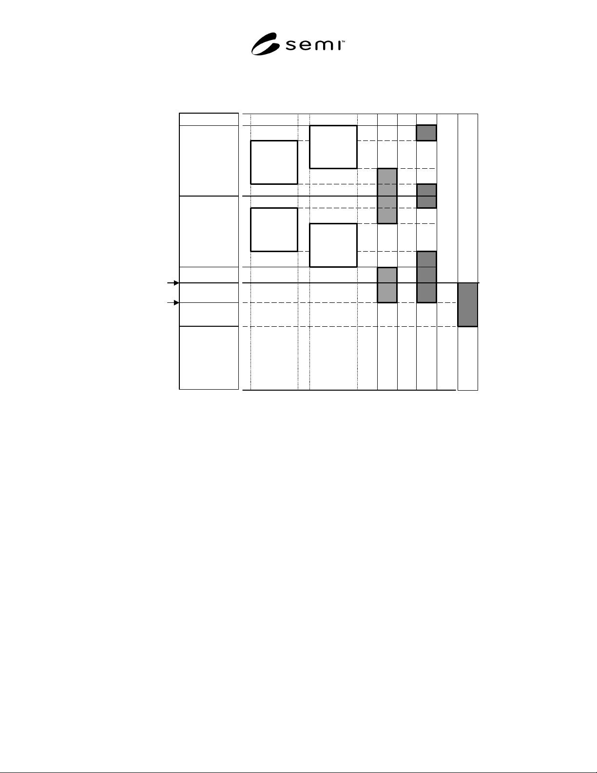
Figure A2-2
Productivity Losses Included in PEE and DEE, and IEE Metrics (shaded regions)
NOTICE: SEMI makes no warranties or representations as to the suitability of the standard set forth herein for any
particular application. The determination of the suitability of the standard is solely the responsibility of the user.
Users are cautioned to refer to manufacturer’s instructions, product labels, product data sheets, and other relevant
literature respecting any materials mentioned herein. These standards are subject to change without notice.
The user’s attention is called to the possibility that compliance with this standard may require use of copy-righted
material or of an invention covered by patent rights. By publication of this standard, SEMI takes no position
respecting the validity of any patent rights or copyrights asserted in connection with any item mentioned in this
standard. Users of this standard are expressly advised that determination of any such patent rights or copyrights, and
the risk of infringement of such rights, are entirely their own responsibility.
SEMI E79-0304 © SEMI 1999, 2004 18
RELATED INFORMATION 1
GUIDELINES FOR DETERMINING THEORETICAL PRODUCTION TIME
PER UNIT
NOTICE: This related information is not an official part of SEMI E79. This related information was approved for
publication by vote of the responsible committee on December 15, 1999.
R1-1 Background
R1-1.1 Overall Equipment Efficiency (OEE) is
computed in terms of the theoretical production time
per unit for each recipe performed. This theoretical time
per unit is based on the actual recipe, the actual
equipment design in use, and an assumed load size that
optimizes equipment throughput (expressed in units of
output per hour) for that recipe.
R1-1.2 OEE is intended to express the true efficiency
of the equipment resource. A score of 50% OEE
indicates that exactly half of the maximum productive
potential of the equipment resource is being realized; a
score of 100% indicates that no further increase in
productivity is feasible, taking the existing process
recipes and equipment design as given.
R1-1.3 To accurately calculate OEE in turn requires
that theoretical production times per unit be accurately
defined. In particular, theoretical production times per
unit shall be defined so that the speed losses are always
non-negative, i.e.,
Speed Losses
= (Production Time) - (Theoretical Production Time for
Actual Units) ≥ 0
R1-1.4 According to now-classical industrial
engineering practice, standards for ideal performance
are determined by application of the following:
• Break work methods down into their operational
elements (hereafter simply referred to as elements).
• Study each of these elements separately to
determine its ideal duration.
• Design a new ideal method offering the shortest
sequence of only the necessary elements (where the
term “sequence” as used herein may involve
parallel performance of some or all elements).
R1-1.5 It is remarked that even when the durations of
all elements are ideal, if the sequence of elements is not
ideal, ideal overall performance cannot be achieved.
Based on this understanding, theoretical processing
time for an equipment recipe shall be based on both an
ideal element sequence as well as ideal durations for all
elements.
R1-2 Modeling Operational Element
Sequences
R1-2.1 A graphical model of the sequence of
operational elements comprising the performance of an
equipment recipe can be helpful for determining
theoretical production time per unit. This model has the
following components:
R1-2.2 Resource Utilization Chart — a Gantt chart
displaying a separate timeline for each primary resource
within the equipment. Utilization sequences displayed
for each primary resource may be used to show how
each resource within an equipment system is utilized,
and how resources may interact.
R1-2.3 Operational Element — An operational
element occurring within a utilization sequence is
depicted by a box-shaped bar with a label. The time for
this element to execute may be fixed, recipe-dependent,
or calculated from parameters. Operational elements
that are not related to material handling operations have
a thick outline.
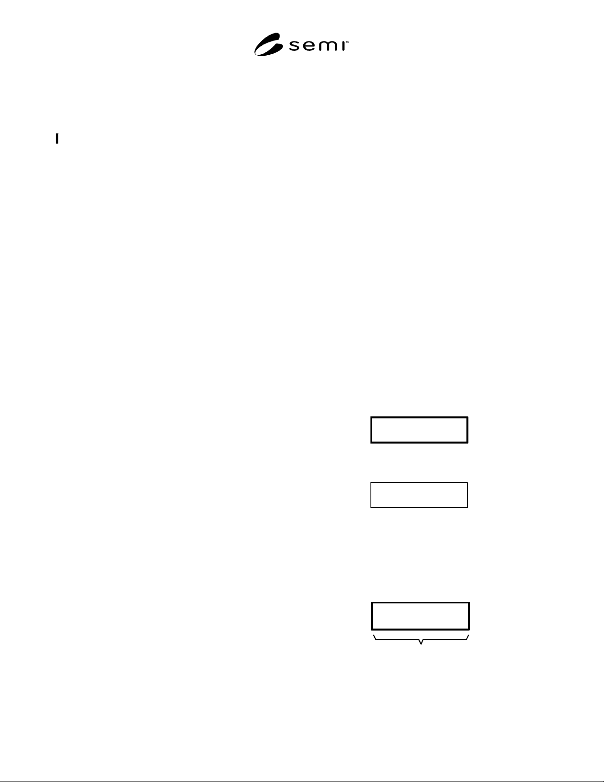
Operational Element
R1-2.3.1 Material handling elements have a thin
outline.
Material Handling
Operational Element
R1-2.4 Repeated Groups — A bracket underneath a
group of operational elements indicates that the group
repeats multiple times based on the parameter shown.
For elements that occur conditionally, the number of
repetitions may be zero. These repetitions apply to all
elements in all timelines positioned in the vertical range
of the bracket.
Repeated
Operational Element(s)
x (# repetitions)
R1-2.5 Sub-Sequences — A number in front of an
element label indicates that the element represents a

SEMI E79-0304 © SEMI 1999, 2004 19
group of elements defined elsewhere. This group is
referred to as a sub-sequence.
1.1 Sub-Sequence
Operational Element
R1-2.6 Calculating Theoretical Production Time Per
Unit — Any element sequence may be modeled as an
activity-on-node network derived from precedence
constraints on the operational elements and precedence
constraints on the allocation of equipment resources to
the elements. Using the network model, the duration of
the element sequence is simply the duration of the
critical path through the network.
R1-2.6.1 Theoretical production time per unit is then
the theoretical duration for the element sequence
divided by the number of units processed during the
sequence.
Theoretical Production Time Per Unit for recipe i [THT
i
]=
= (Theoretical Duration for the Element Sequence)
/(Number of Units Processed During Sequence)
R1-2.7 Allowances for Non-Steady-State Processing —
For complicated batch-load equipment models, it is
useful to divide resource sequences into a beginning
phase, a steady-state-phase, and an ending phase. For
modeling theoretical time, it is important to determine
what allowances to make, if any, for the beginning and
ending phases. For machines that are limited in the
number of lots that can be processed in a continuous
cascade, appropriate allowances shall be made for
beginning and ending phases. However, for machines
that are capable of running continuously, the beginning
and ending phases should not be considered in
determining theoretical production time.
R1-2.7.1 Under certain conditions, setup type
operations that are not tracked as part of downtime shall
be considered as part of the theoretical resource
sequence for a tool. These conditions include
operations that shall occur in every machine cycle, e.g.
recipe download, as well as operations that occur on
other regular intervals, e.g., one clean cycle every 75
wafers. In general, any activity that occurs on
predictable intervals and is a necessary part of a recipe
specification should be considered in the equipment
sequence for determining theoretical production time.
R1-2.7.2 Operations that occur at irregular intervals or
that apply to an unpredictable quantity of wafers, lots,
or loads are not counted. An example of an
unpredictable frequency setup is a recipe changeover,
when the machine is changed from the requirements of
one process recipe to meet the needs of another, e.g., a
species change as on an ion implant system. The ideal
frequency of these events is taken as zero.
R1-2.8 Optimality — Theoretical sequences shall be
designed so as to optimize equipment throughput by
using only the best configuration of elements and an
optimal load size. Optimal sequences may differ for
different recipes performed on the same machine.
Optimal load sizes are not necessarily maximum load
sizes.
R1-2.9 Error-Checking Element Sequences Once a
theoretical sequence is specified for a piece of
equipment, it can be compared against actual equipment
operations to check for errors. If discrepancies are
found, three possibilities to investigate are:
• The sequence contains extraneous elements.
• The sequence is missing necessary elements.
• The series and parallel relationships between
elements are not correctly specified.
R1-2.9.1 What may at first appear to be sequence
specification errors may in fact be undiscovered rate
efficiency losses embedded in the equipment sequence.
Because sequences are fundamental to overall
performance, it is important to rule out sequence
specification errors to preclude erroneous assignment of
rate efficiency losses to individual elements.
R1-2.10 Example Resource Utilization Sequence An
example of a resource utilization sequence is given in
Figure R1-1. This example represents a particular
instance of a photolithography stepper that exposes
patterns from a reticle onto a wafer. This example
assumes that the stepper receives individual unexposed
wafers from a linked coat track and transfers individual
exposed wafers to a linked develop track.
R1-2.10.1 First, a reticle box shall be loaded into the
stepper reticle handling system (“load box”). Before a
wafer may be exposed, the reticle shall be set and
aligned. A wafer shall also be loaded onto the pre-align
chuck, pre-aligned, and transferred to the exposure
stage. Each wafer is exposed then transferred to a post
processing relay chuck. The transfer operation
simultaneously removes an exposed wafer and replaces
it with an unexposed wafer.
R1-2.10.2 The expose operation is represented by the
sub-sequence shown in Figure R1-2. Depending on the
recipe to be executed, the expose sub-sequence may
consist of several different reticle images requiring
changes of “blade” positioning. For each image, there is
one “align” operation. For each individual exposure,
there is a “step” operation, a “level” operation, and the
“expose” operation itself. Within the same image,
different exposures may require different leveling
times, as well as different stepping times.