semi合集-English.pdf - 第463页
SEMI E66-1103 © SEMI 1997, 2003 12 A1-1.3 Figure A1-2 gives an ove rall picture of the data collection s pecified by Table A2-1 for both “BACKGROUND” and “DEVICE”. T h ere are three phases of data collectio n: 1. Cleanu …
SEMI E66-1103 © SEMI 1997, 2003 11
APPENDIX 1
STATISTICAL PROCESS CONTROL CHARTING
NOTE: This appendix was approved as an official part of SEMI E66 by full letter ballot procedure.
A1-1
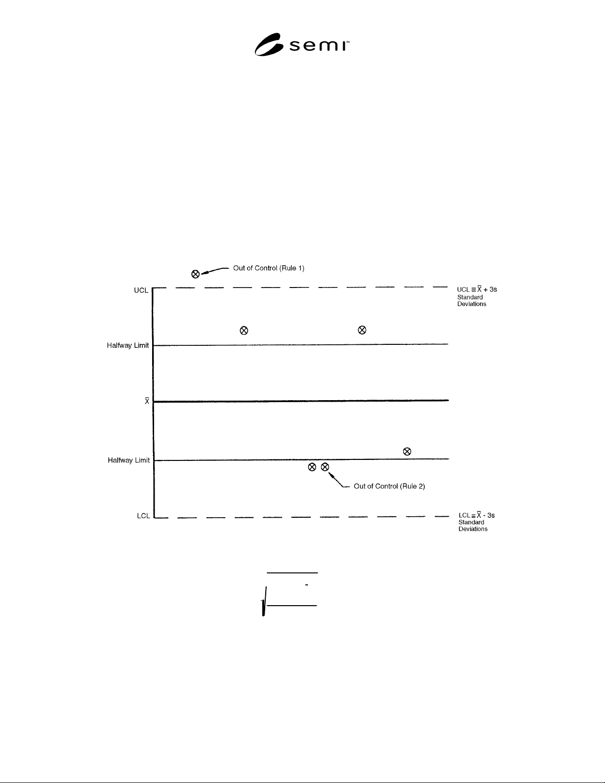
A1-1.1 The following rules should be used to interpret the statistical process control chart, Figure A1-1:
1. If one observation is outside UCL/LCL, the process is out of control.
2. If two consecutive observations are > halfway, the process is out of control.
3. If at least eight successive points are in control, the process is stable.
A1-1.2 It has been assumed that the data is approximately normal under log transform and that samples are
independent.
Figure A1-1
Statistical Process Control Chart
S =
(x
i
−
x )
2
1
n
∑
n − 1
where n = # of observations
SEMI E66-1103 © SEMI 1997, 2003 12
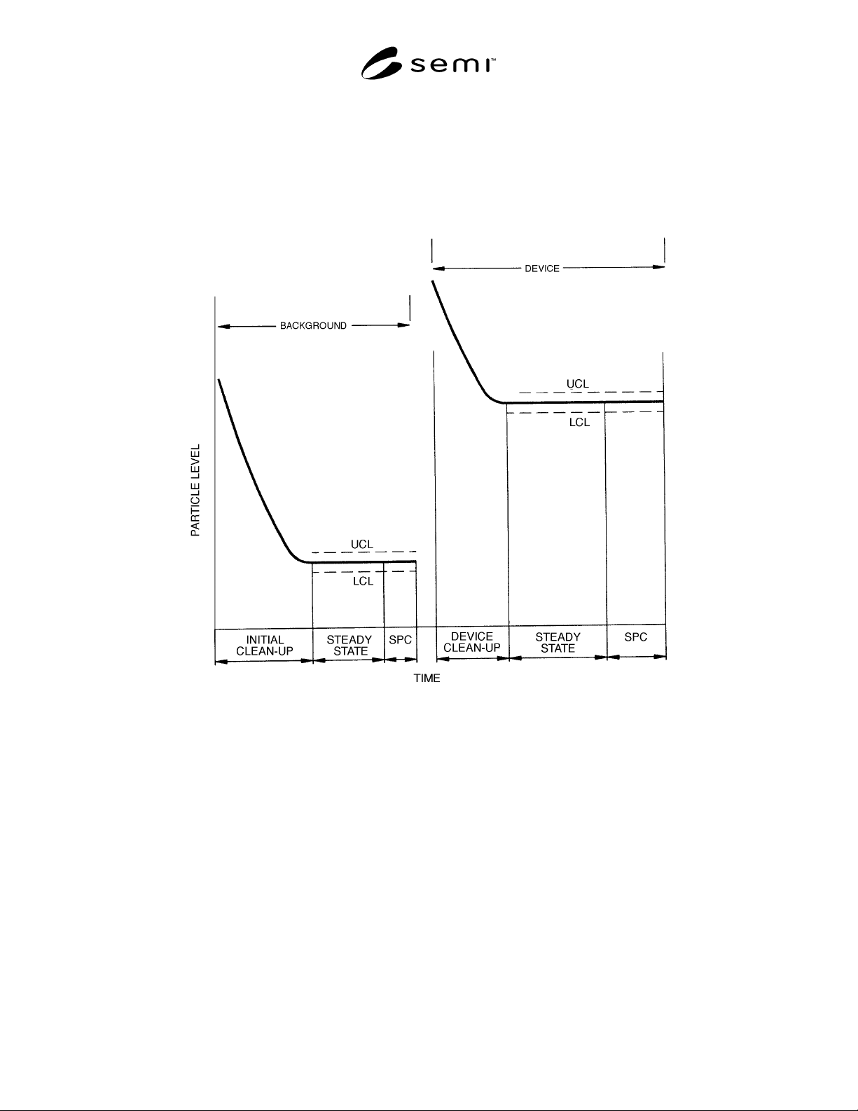
A1-1.3 Figure A1-2 gives an overall picture of the data collection specified by Table A2-1 for both
“BACKGROUND” and “DEVICE”. There are three phases of data collection:
1. Cleanup
2. Steady-state performance
3. Statistical process control (SPC)
Figure A1-2
Graphical Representation of Data Collection
SEMI E66-1103 © SEMI 1997, 2003 13
APPENDIX 2
t-TESTING; COMPARISON OF BACKGROUND MEAN AND DEVICE
MEAN
NOTE: This appendix was approved as an official part of SEMI E66 by full letter ballot procedure.
A2-1
A2-1.1 The background and DUT are expected to have low particle counts. Therefore, a statistical method is needed
to determine if there is a difference between background and DUT particle counts. The t-test is a method of
determining the actual statistical difference between the mean background particle count and the mean device
particle count. It can be used to characterize the particle contribution by the MFC Record results in Table A2-1.
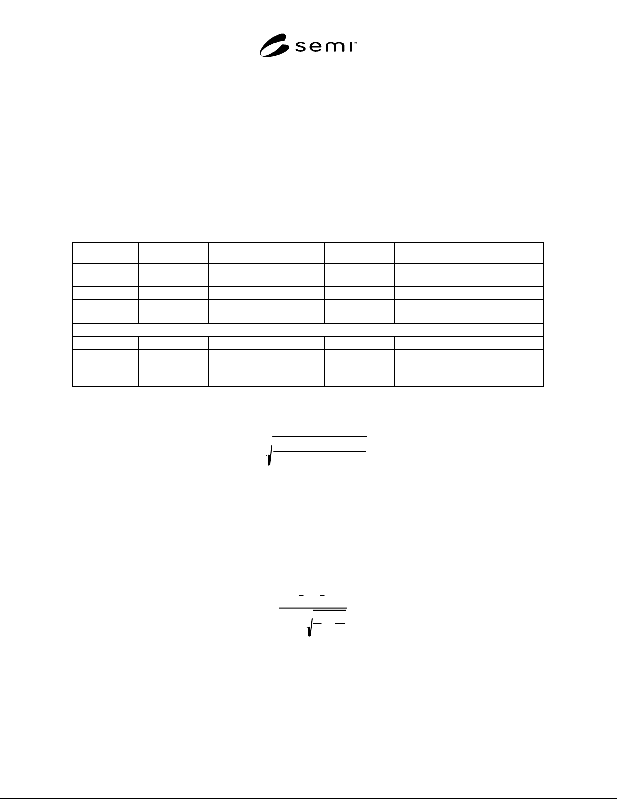
Table A2-1 Test Worksheet
# Observation log Observation Remarks
Spool Cleanup 1 ... Nx All computations are in the logs of
original observations.
Stable Level X1 ... X25 Compute X
1, S1, UCL, LCL.
SPC X26 ... X334 Use all 8 values to recompute new
values (X
1,S1
).
Connect Device
Device Cleanup X34 ... X35 + n
Stable Level X34 + n + 1 ... X34 + n + 25 Compute X
2, S2, UCL, LCL
.
SPC X34 + n + 26 ... X34 + n + 34 Use all 8 values to recompute new
values (X
2, S2
).
NOTE: Use t-test to compare X’s. (See Appendix 2.)
A2-1.2 Calculate pooled standard deviation using the following equation:
S
pooled
=
(n
1
− 1)S
1
2
+ (n
2
− 1)S
2
2
n
1
+ n
2
− 2
where :
S
1
= background standard deviation
S
2
= device standard deviation
n
1
= background sample size
n
2
= device sample size
A2-1.3 Calculate the value of T (the t-test’s namesake) as follows:
t =
X
1
− X
2
S
pooled
1
n
1
+
1
n
2
where :
1 = background mean
2 = device mean