semi合集-English.pdf - 第5167页
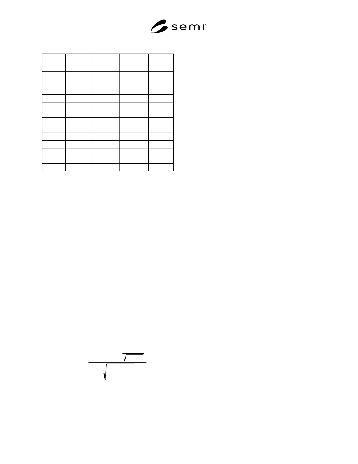
SEMI M32-0998 © SEMI 1998, 2004 6 Table A2-1 Lognormal v s. Normal Data Value Value Description Normal ppm > Lognormal ppm > Error 1.8263 mean 500000 420997 79003 2.5831 + 1 s 158655 141869 16786 3.3399 + 2 s 22750…
SEMI M32-0998 © SEMI 1998, 2004 5
APPENDIX 2
USING STATISTICAL SPECIFICATIONS FOR LOGNORMAL
PROCESSES
NOTICE: This appendix was approved as an official part of SEMI M32 by full letter ballot procedure.
A2-1 Statistical Specification Format for
Lognormal Distributions
A2-1.1 The lognormal probability distribution function
describes many of the one-sided distributions
encountered in the silicon industry. It applies to those
one-sided parameters like flatness and warp that are
bounded by zero. Below is an example of a statistical
specification for a lognormal process.
≤ xx @ yy ppm
A2-1.2 Other standard tolerance definitions could be
substituted, or other quality level definitions such as
ECPK, Z-value, or percent could be used. Again, ECPK
is the Equivalent normal Cpk that corrects for non-
normality. More information on the Equivalent Cpk is
shown at the end of this appendix.
A2-1.3 As with the normal distribution, adding the
quality level removes the potential for
misunderstanding and makes the specification more
meaningful.
A2-2 Example of Use
A2-2.1 Again, the major objectives are to focus quality
improvement efforts, achieve ship-to-stock
relationships, promote processed in quality, and reduce
after the fact inspection. The steps are the same as
shown in Section A1-2 for the normal distribution. The
major difference is that only the upper tail needs to be
considered. However, since the lognormal tail goes so
much farther out, it might be necessary to accept a less
critical quality level.
A2-3 Discussion
A2-3.1 Statistical specifications work very well for
processes with lognormal distributions. They have all
the benefits described for normal distributions, and in
some respects, they are even easier. Since lognormal
processes only have one tail, checking each tail to
decide which is the most critical is not necessary. Also,
it has been empirically observed that lognormal
processes are not as prone to mean drifting, so they tend
to be more stable. The main hurdle is realizing how
much error is introduced if the distribution shape is
assumed to be normal when it is not.
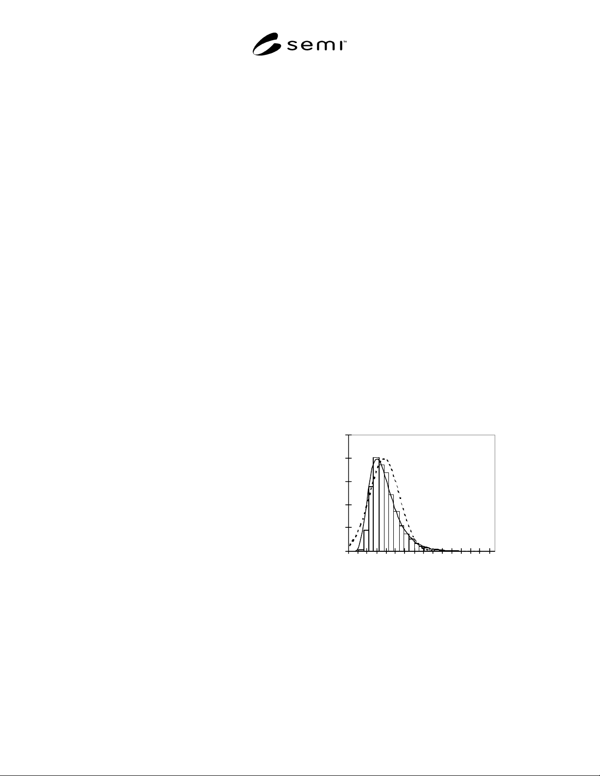
A2-3.1.1 Figure A2-1 illustrates the difference between
a lognormal and a normal process. The curve which has
a solid line (and is clearly not symmetrical) is the
lognormal distribution. The curve with the dashed line
is the normal distribution. The error when mistakenly
using a normal distribution to characterize a lognormal
process is shown in Table A2-1. For values that
increment by 1 sigma from the mean, the ppm greater
than that value is given for each curve, and the
difference (or error) is calculated. To make it easier to
visualize, increments of the simple normal mean and
sigma (1.8263 and 0.7568 respectively) are used in the
“value” column. For calculating the lognormal statistics
the correct lognormal geometric mean of 1.8258 and
the lognormal geometric sigma of 0.7550 are used. The
error between the curves increases as the point of
interest moves toward the center of the distribution, but
the most important issue is the length of the tail. The
right tail of the lognormal distribution extends along
with the histogram, but the normal distribution is much
shorter. Visually, the significance might be overlooked
in Figure A2-1, but when the tail probabilities are
shown in ppm (Table A2-1) the difference is very
apparent.
0
500
1000
1500
2000
2500
0.0 1.0 2.0 2.9 3.9 4.8 5.8 6.7
Figure A2-1
Lognormal vs. Normal Curves
SEMI M32-0998 © SEMI 1998, 2004 6
Table A2-1 Lognormal vs. Normal Data
Value
Value
Description
Normal
ppm >
Lognormal
ppm >
Error
1.8263 mean 500000 420997 79003
2.5831 + 1 s 158655 141869 16786
3.3399 + 2 s 22750 42836 20086
4.0967 + 3 s 1350 12783 11433
4.8535 + 4 s 32 3914 3882
5.6103 + 5 s 0.3 1247 1247
6.3671 + 6 s 415 415
7.1239 + 7 s 144 144
7.8807 + 8 s 52 52
8.6375 + 9 s 20 20
9.3943 + 10 s 8 8
10.1511 + 11 s 3 3
10.9079 + 12 s 1 1
A2-3.2 Lognormal distributions can be handled
mathematically as easily as normal distributions, if the
formulas are known. The difficulty in the past was that
many of the calculations developed for the normal
distribution were not available for lognormal. The
equivalent normal Cpk (ECPK) was developed to
address this issue. For the lognormal distribution,
ECPK is calculated as shown below. It is an exact
mathematical derivation with no estimations or
assumptions. It was designed to allow people to see real
data and keep all transformations and conversions
inside the computer where they are totally invisible.
Two cases are presented. Section A2-3.3 describes the
case where a statistical software is available, and
Section A2-3.4 describes a shortcut that may be used
when the computation is derived from scratch. In both
cases, it is important to remember that only the
computer will see these formulas.
A2-3.3 Statistical software packages will usually
output the geometric mean and geometric sigma. If µ is
the lognormal geometric mean, σ is the lognormal geo-
metric sigma, and 1n is the natural log function, then
ECPK is calculated as:
ECPK =
1n [USL]−1n
µ
2
µ
2
+
σ
2
31n
µ
2
+
σ
2
µ
2
For the example in Figure A2-1 the lognormal
geometric mean is 1.826 and the lognormal geometric
sigma is 0.755. If an upper spec limit (USL) of 6 is
applied, then the ECPK is 1.06. This will usually be
done in a computer. A programming version of this
formula is written as:
ECP
K
= ((log (USL))
−
log (Gmea
n
**2 / (sqr
t
(Gmean **2 + Gsigma **2)))) / (3* sqrt (log
((Gmean **2 + Gsigma**2) / Gmean* *2)))
A2-3.4 If the computation is programmed from scratch
for raw data, it may be convenient to take the natural
log of each data point (i.e., do a log transformation)
then compute the mean of the transformed data
(Tmean) and sigma of the transformed data (Tsigma).
Again, ln is the natural log function. In this case, the
ECPK formula can be written as:
ECP
K
= (1n(USL)
−
Tmean)/(3* Tsigma)
The geometric mean and geometric sigma could then be
calculated as follows:
Gmea
n
= exp(Tmea
n
+(Tsigm
a
* *2)/2)
Gsigma = sqrt((exp((2 * Tmean) + (Tsigma * *2)))*
(exp((Tsigma * *2)) − 1))
A2-4 Conclusion
Lognormal calculations can be as easy as normal
calculations. Again, the formulas reside only in the
computer where they are never seen by the user. They
allow the user to view the actual measures and the
actual distributions.

SEMI M32-0998 © SEMI 1998, 2004 7
APPENDIX 3
CURRENT STATISTICAL CHARACTERIZATION OF SILICON
PROCESS PARAMETERS
NOTICE: This appendix was approved as an official part of SEMI M32 by full letter ballot procedure.
A3-1 Statistical Characterization of Silicon Process Parameters
A3-1.1 The following table describes the statistical characterization on a number of silicon wafer processes. The
comments column indicates the level of characterization that has been achieved. “Characterized” means that the
process should, under usual conditions, display the distribution shape shown. “Conditional” means that there are
conditions that might need to be considered before deciding if the shape shown is satisfactory. The chi-square
goodness of fit test was used to characterize the distribution shapes. Actual chi-square goodness of fit values will
typically be proprietary information that is shared only between a given supplier and user.
Table A3-1 Characterization of Silicon Processes
Process or Parameter
Description
Distribution
Shape
Comments
Diameter Normal Characterized
Flatness/Global (GBIR, GF3R, GF3D, GFLR, or GFLD) Lognormal Characterized
Flatness/Site (SF3R, SF3D, SFLR, SFLD, SFQR, SFQD, SBIR,
or SBID)
Lognormal Characterized
Oxygen Concentration Normal Conditional — Non-normalities are mostly
attributed to measurement error, so the
normal distribution is usually satisfactory.
Shape, Bow (Reference SEMI M1, Figure A2-1.) Normal Characterized
Shape, Warp, or Sori (Reference SEMI M1, Figure A2-1.) Lognormal Characterized
Thickness (Polished or EPI) Normal Characterized