semi合集-English.pdf - 第5240页
SEMI M40-0200 © SEMI 2000 22 R1-5. 3.2 Wafer roughne ss ma ps wit h 1 mm 2 pixel size were generated using all possible 3 2 combinations of the parame ters in T able R1-5. Av erage roughness an d standard deviation we re…

SEMI M40-0200 © SEMI 200021
Table R1-7 Normalized values of Table R1-6
Variable Set # ravg1 ravg5 ravg9 rstdabw5 rstdabw9
1 1.0000 1.0000 1.0000 0.0000 0.0000
2 1.6000 1.1440 1.0160 0.1920 0.1360
3 0.8000 0.9360 1.0320 0.0560 0.1440
4 1.3333 1.0667 1.0400 0.3267 0.3333
5 0.8000 0.9840 0.9280 0.1120 0.0320
6 1.3333 1.1000 0.9533 0.0800 0.0600
7 0.6667 0.9333 0.9600 0.1400 0.1400
8 1.1429 1.0457 0.9771 0.0400 0.1029
9 0.8000 0.9360 1.0320 0.0560 0.1440
10 1.3333 1.0667 1.0400 0.1400 0.1400
11 0.6667 0.9000 1.0467 0.0800 0.0600
12 1.1429 1.0114 1.0514 0.0800 0.0229
13 0.6667 0.9333 0.9600 0.3267 0.3333
14 1.1429 1.0457 0.9771 0.0400 0.1029
15 0.5714 0.8971 0.9886 0.1371 0.0971
16 1.0000 1.0000 1.0000 0.0000 0.0000
17 1.0000 1.0000 1.0000 0.0000 0.0000
18 1.4085 1.1127 1.0775 0.2676 0.2746
19 0.9259 0.9444 0.9444 0.0556 0.0556
20 1.3333 1.0667 1.0400 0.3267 0.3333
21 0.7042 0.9366 0.9155 0.2183 0.1761
22 1.0811 1.0324 0.9892 0.0541 0.0108
23 0.6667 0.9000 0.8800 0.2533 0.2133
24 1.0417 1.0052 0.9635 0.0000 0.0365
25 0.9259 0.9907 1.0556 0.0000 0.0648
26 1.3333 1.1000 1.1200 0.2533 0.2133
27 0.8696 0.9478 1.0174 0.0870 0.0174
28 1.2658 1.0570 1.0759 0.1962 0.1582
29 0.6667 0.9333 0.9600 0.3267 0.3333
30 1.0417 1.0313 1.0313 0.0313 0.0313
31 0.6329 0.8987 0.9304 0.2405 0.2468
32 1.0000 1.0000 1.0000 0.0000 0.0000
average 0.9968 0.9987 1.0001 0.1287 0.1254
standard deviation 0.2700 0.0682 0.0521 0.1106 0.1080
maximum 1.6000 1.1440 1.1200 0.3267 0.3333
minimum 0.5714 0.8971 0.8800 0.0000 0.0000
SEMI M40-0200 © SEMI 2000 22
R1-5.3.2 Wafer roughness maps with 1 mm
2
pixel size were generated using all possible 32 combinations of the
parameters in Table R1-5. Average roughness and standard deviation were calculated by using all pixels of a map
(avgtrue, stdabwtrue) as well as by using the three discrete site patterns displayed in Figure 1 of the main part of this
document (avg1, avg5, avg9, stdabw5, stdabw9). Corresponding results for comparing models a and b are displayed
in Table R1-6. These values were normalized for further evaluation, the averages with respect to avgtrue
(ravgi=avgi/avgtrue, i=1,5,9), the standard deviations with respect to their difference to the “true” value
((rstdabwi=stdabwi.-stdabwtrue) / stdabwtrue, i=5,9) (Table R1-7). Results for comparing models a and c are
similar and are not reported here in detail.
R1-5.3.3 The averages for ravg1,5,9 over the various variable sets differ by less than 1% from unity. The
corresponding standard deviations decrease from 27% to 5% going from ravg1 to ravg9, respectively, indicating
as one would expect that ravg9 is a much more precise value for the roughness of the entire surface as compared
to ravg1 or ravg5. The relative standard deviations rstdabw5,9 deviate in the average by about 12% from the true
value. The corresponding standard deviations differ not much for rstdabw5 and rstdabw9.
R1-5.3.4 More detailed information is obtained when the results are evaluated according to the factorial design
used. The 1
st
to 5
th
order effects of varying the variables were calculated by applying using a table of contrast
coefficients /10/ to the normalized results of the simulation. The 1
st
order or main effects are the difference of
the observations for both levels of one parameter and averages over all other observations. They measure the
average effect of a variable over all conditions of the other variables. The 2
nd
order effects are a measure for the
interaction of variables and are obtained by calculating one half of the difference of the average effect of variable 1
with variable 2 at level 1 and variable 1 with variable 2 at level 2. 3
rd
order and higher effects are not considered in
the present work. They are assumed to be negligible and are used to calculate the variance of an effect (=square root
of the average of the squares of 3
rd
to 5
th
order effects).
R1-5.3.5 The result of this evaluation is displayed in Table R1-8 and Table R1-9 for the main (1
st
order) and 2
nd
order effects, respectively.
Table R1-8 Average (over all sets of variables) and Main Effects of the Various Variables on the
Observables (The variance as calculated from the 2
nd
to 5
th
order effects is displayed in the last column.)
Average
c1 e1 c2 e2 Sym. Variance
ravg1 0.9968 0.4482 -0.1111 -0.2237 -0.1111 -0.0064 4.16E-05
ravg5 0.9987 0.1134 -0.0460 -0.0377 -0.0287 -0.0027 3.69E-06
ravg9 1.0001 0.0439 -0.0067 -0.0734 0.0356 -0.0001 4.37E-06
rstdabw5 0.1287 -0.0038 -0.0049 -0.0073 -0.0080 0.0315 3.43E-04
rstdabw9 0.1254 -0.0064 -0.0057 -0.0113 -0.0052 0.0198 4.87E-04
Table R1-9 2
nd
Order Effects (The variance as calculated from the 2
nd
to 5
th
order effects is displayed in the
last column.)
c1/e1 c1/c2 c1/e2 c1/sym e1/c2 e1/e2 e1/sym c2/e2 c2/sym e2/sym Variance
ravg1 -0.0157 -0.0221 -0.0157 -0.0590 0.0218 0.0160 0.0579 0.0218 -0.0547 0.0579 4.16E-05
ravg5 -0.0015 -0.0079 -0.0040 -0.0067 0.0065 0.0054 0.0064 0.0039 -0.0225 0.0238 3.69E-06
ravg9 -0.0003 0.0023 -0.0057 0.0304 0.0049 -0.0015 -0.0304 -0.0005 -0.0092 0.0119 4.37E-06
rstdabw5 -0.0062 -0.1848 -0.0603 -0.0027 -0.0423 -0.0392 0.0059 0.0335 -0.0005 0.0029 3.43E-04
rstdabw9 0.0080 -0.1471 -0.0722 0.0002 -0.0247 -0.0894 0.0003 0.0518 0.0027 0.0008 4.87E-04
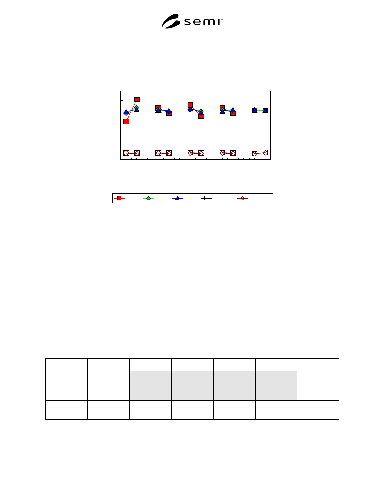
R1-5.3.6 The behavior of the main effects is also illustrated in Figure R1-5, where the variation of ravg1,5,9 and
stdabw5,9 are plotted vs. the variables. The clear effect, on ravg1, of varying center1 between 0.1 and 0.2 is easy to
understand as ravg1 consists only of one measurement point in the center of the wafer surface. Similar but less
pronounced effects are observed for ravg5 and 9. Note that the opposite effect occurs for center 2 as this point is not
included in calculating ravg1,5 or 9. Also note that the influence of the variables edge1 or edge2 is much less
SEMI M40-0200 © SEMI 200023
pronounced. In any case, the 5-point measurement provides the correct average ± 6%, the 9-point measurement ±
2.5%. In a similar way, the 5-point standard deviation is correct ± 1.6% and the 9-point standard deviation ± 1%.
0
0.2
0.4
0.6
0.8
1
1.2
1.4
center1 lo
center1 hi
edge1 lo
edge1 h i
center2 lo
center2 hi
edge2 lo
edge2 hi
sym. rot.
sym. cyl
Variables
Effects
ravg1 ravg5 ravg9 stdabw5 stdabw9
Figure R1-5
Main Effects of the 2
5
Factorial Design for Models a and b
R1-5.3.7 The significance of numbers given in Table R1-8 and Table R1-9 can be estimated only in relation to the
noise or variance of the observables which is also displayed in both tables. The signal-to-noise ratio S/N is obtained
by using a logarithmic measure:
S/N = 10 log (effect
2
/variance)
R1-5.3.8 The corresponding S/N values for the main and for the second order effects are listed in Table R1-10 and
Table R1-11.
R1-5.3.9 A linear signal-to-noise ratio of 3:1 is commonly used to distinguish significant data from insignificant
data. This linear ratio corresponds to a S/N of about 10 in the present case of a logarithmic signal-to- noise ration.
The S/N ratios > 10 are shaded lightly gray in Table R1-10 and Table R1-11. The variables center1,2 and edge1,2
have a significant effect on the relative averages ravg1,5,9. Mainly the interactions of the model selected with the
other variables are significant for the relative averages ravg1,5,9 and the interaction of center1 and center2 for the
relative standard deviations rstdabw5,9. The other cases emphasized in Table R1-11 by shading have a S/N ratio
only slightly larger than 10.
Table R1-10 S/N Ratios for the Main Effects of Table R1-8
average c1 e1 c2 e2 Sym
ravg1 43.7817 36.8384 24.7251 30.8046 24.7251 -0.0364
ravg5 54.3215 35.4230 27.5959 25.8609 23.4801 2.9416
ravg9 53.5959 26.4387 10.1741 30.9124 24.6260 -26.2612
rstdabw5 16.8383 -13.6750 -11.4959 -8.0646 -7.3246 4.6154
rstdabw9 15.0934 -10.7996 -11.7656 -5.7926 -12.5745 -0.9359