semi合集-English.pdf - 第6607页
SEMI C10-0305 © SEMI 1998, 2005 4 s 2 / 1 xx SS 2 X n 1 1 0013 . 0 , 2 n t b UCL n i i Y Y and n i i X X where (3), X m Y b 2 n i i X i 2 i X 2 i X i X xx SS and summations in the 1 by to 1 f…
SEMI C10-0305 © SEMI 1998, 2005 3
6.3.2.5 Ordinary Least Squares (OLS) — A curve-fitting criterion which, for a given calibration model, minimizes.
2
1
Pr
n
i
i
Yedicted
i
Y
Appropriate use of this criterion implicitly assumes that, on average, each determination is made with equal
reliability.
6.3.2.6 Weighted Least Squares (WLS) — A curve-fitting criterion which, for a given calibration model, minimizes.
.point data the toassigned weight theis where,
2
1
Pr
th
i
i
w
n
i
i
Yedicted
i
Y
i
w
Appropriate use of this criterion implicitly assumes that all w
i
are strictly inversely proportional to each point's
standard deviation (measure of variation).
6.3.2.7 t-statistic — Student’s t is used instead of the Z-statistic (normal distribution) when the standard deviation is
estimated from relatively small quantities of data. It is used herein to explicitly control the risk at 0.13%, regardless
of sample size.
Xs — The concentrations of the standards used in quantifying the MDL.
Ys — The instrument’s response (signal intensity) to each of the Xs in question.
6.3.3 Calculations — OLS and Linear Calibration Model
6.3.3.1 A line, which is not constrained to pass through the origin, is used as the calibration model. OLS is used to
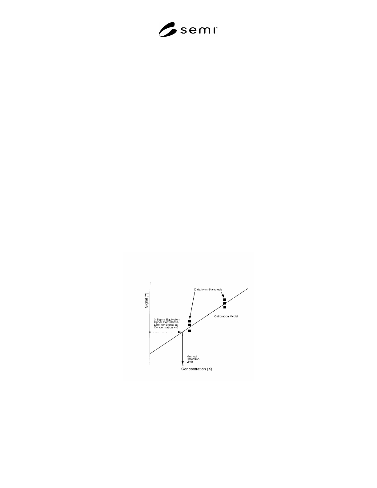
estimate the model. The MDL is located by determining the 3 sigma equivalent Upper Confidence Limit at X = 0
and using a linear calibration model to convert this result into the corresponding concentration (MDL).
Figure 1
Graphical Visualization of MDL
Determination Process

SEMI C10-0305 © SEMI 1998, 2005 4
s
2/1
xx
SS
2
X
n
1
1
0013.0 ,2n
tbUCL
n
i
i
Y
Y
and
n
i
i
X
X
where(3),
XmYb
2
n
i
i
X
i
2
i
X
2
i
X
i
X
xx
SS
and summations
in the 1by to1 from rangesh index whican
is and nsobservatio ofnumber total where
n
i
i
Y
i
i
X
i
Y
i
i
X
Y
i
Y
i
X
i
X
xy
SS
and Squares of Sumfor stands where(2),
xx
SS
xy
SS
m
4)(equation 0 at Limit
Confidence Upper equivalent sigma 3
3)(equation
analysis OLSby determinedintercept
2)(equation
analysis OLSby determined slope
where,(1)
m
bUCL
MDL
n
in
SS
X
UCL
b
m
SEMI C10-0305 © SEMI 1998, 2005 5
b
i
mX
*
i
Y where,
2/1
2n
i
2
*
i
Y
i
Y
model regression ofdeviation standard s
and )equivalent sigma 3 sided,-(one signal
positive false a detecting ofrisk desired theas
0.0013 and freedom of degrees 2 n with
1) Table (from statistic - t a is
0.0013 2,
t
where(4),
n
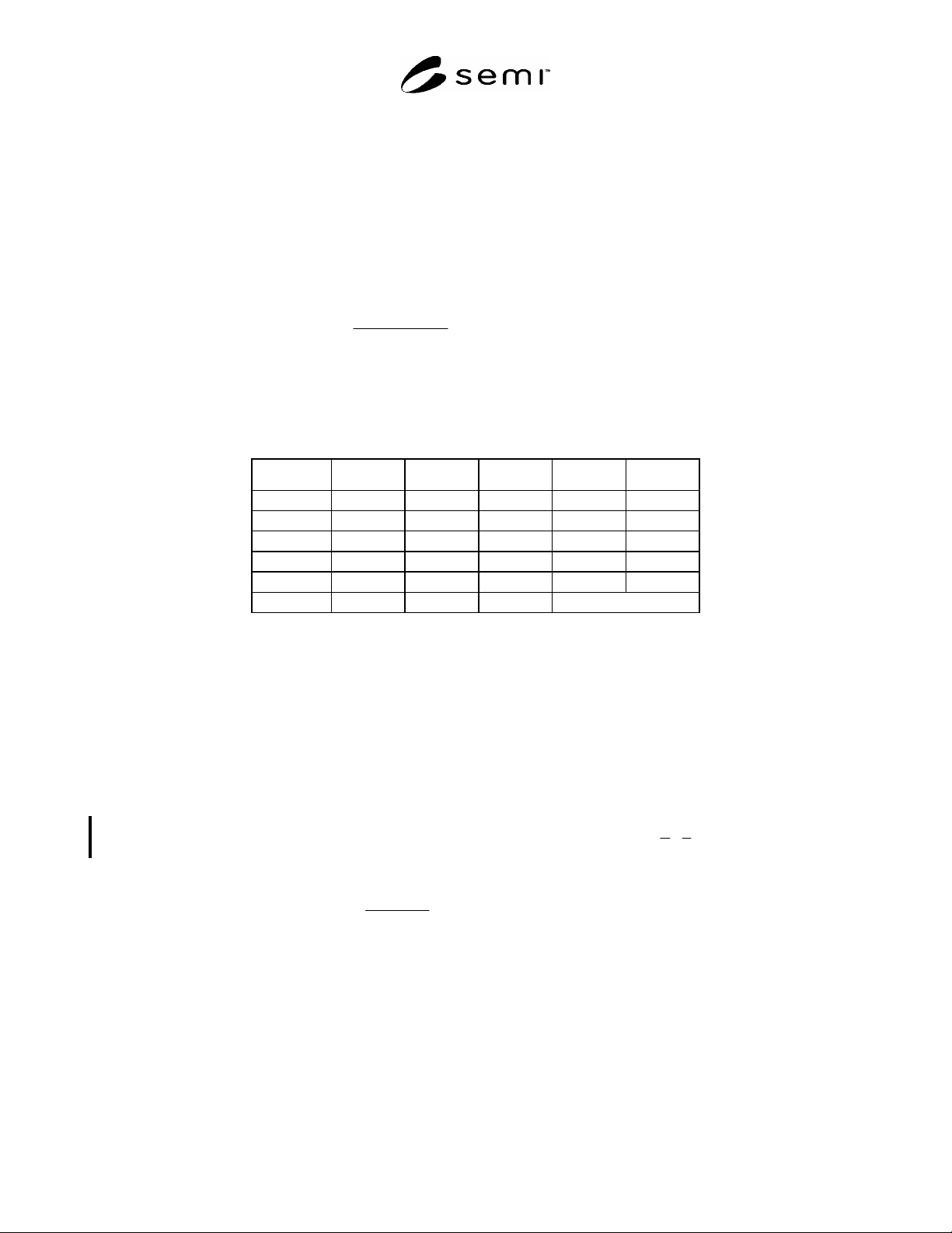
Table 1 3-Sigma Equivalent t-Table
n-2 t n-2 t n-2 t
4 6.62 10 3.96 16 3.54
5 5.51 11 3.85 17 3.51
6 4.90 12 3.76 18 3.48
7 4.53 13 3.69 19 3.45
8 4.28 14 3.64 20 3.42
9 4.09 15 3.59
6.3.3.2 Such analyses should be performed by using a spreadsheet or computer program. It is not recommended to
do them by hand. The previous equations neither require nor prevent use of data from blank quantification. In order
to use blank data in the MDL quantification with OLS, the blank should be measurable, be likely to give a response
which is consistent with the pattern in the other calibration data, and provide a similar level of variability to that
obtained from the investigated standards.
6.3.4 Calculations — WLS and Linear Calibration Model
6.3.4.1 A line which is not constrained to pass through the origin is used as the calibration model. WLS is used to
estimate the model in which the weights are determined as a function of the observed variability at each
concentration level. The MDL is located by determining the 3 sigma equivalent Upper Confidence Limit at X = 0
and using a linear calibration model to convert this result into the corresponding concentration (MDL). While many
of the WLS analysis quantity names are identical to those in the OLS analysis (e.g.,
,X ,Y ), and ,
xy
SS
xx
SS the
calculations are not.
8)(equation WLSusing 0 at
Limit Confidence Upper equivalent sigma 3
7)(equation
analysis by WLS determinedintercept
6)(equation
analysis by WLS determined slope
where, (5)
X
UCL
b
m
m
bUCL
MDL