semi合集-English.pdf - 第5170页

SEMI M32-0998 © SEMI 1998, 2004 9 0 500 1000 1500 2000 2500 0.0 1.0 2.0 2.9 3.9 4.8 5.8 6.7 Figure A4-2 Normal vs. Lognorm al Shape A4-1.7 Statistical sp ecifications quantify the quality level so it is not an abstract a…

SEMI M32-0998 © SEMI 1998, 2004 8

APPENDIX 4

RATIONALE FOR STATISTICAL SPECIFICATIONS

NOTICE: This appendix was approved as an official part of SEMI M32 by full letter ballot procedure.

A4-1 Introduction

A4-1.1 The purpose of a specification is either to

define acceptance criteria or to assist in quality

improvement planning. The basic intent is to quantify

user need so suppliers can accommodate that need.

Developing a clear link between user needs and the

control methods used on the production floor is one of

the most critical steps for creating a Total Quality

Management (TQM) environment. Following are some

key background concepts that allow the reader to

understand the conclusions drawn in this document.

A4-1.2 For most manufacturing processes there is no

such thing as “zero defects”. Processes are described by

statistical probability distributions, and the tails of these

functions can go all the way to infinity. For many years,

99.73% (i.e., ± 3 sigma) was used as the basis for

tolerances. “Within tolerance” was understood to mean

within tolerance with a 99.73% confidence, or a 0.27%

quality level. When users requested better levels, then

new standards such as 33 ppm or 3.4 ppm were made.

In any case, this quality level needs to be agreed upon

for a specification method to have meaning. It can be

measured in terms of ppm, Z, Cpk (which is equal to Z

divided by 3), or percent. Z tables or Cpk tables can be

obtained which provide this information.

A4-1.3 Errors in the 10% or higher range can be

generated if a percentile specification is based on the

central portion of the distribution. An example of such a

specification is “50% ≤ 1.2 microns”. These errors are

not obvious and require careful statistical analysis

based upon real process variation. Multiple percentile

specifications are also difficult to apply. Paragraph A4-

3 provides more details on these issues.

A4-1.4 Conversely, if specifications get too far out on

the tail, they tend to become abstract and are not used

as the primary factor driving quality improvements.

This is especially true for non-normal processes where

the tail of the distribution goes out much farther than

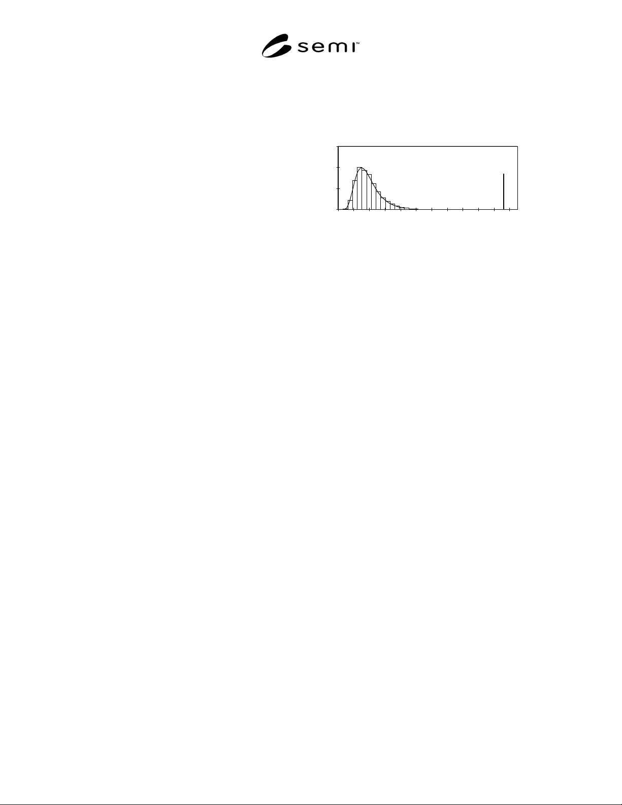
expected from a normal distribution. Figure A4-1

shows where a 3.4 ppm specification would be on a

lognormal process. Users usually will not allow that

much tolerance. However, if the specification is

tightened while the process capability remains the

same, then the consequence is a degradation in the

quality level.

1000

2000

3000

0.0 1.0 2.0 2.9 3.9 4.8 5.8 6.7 7.7 8.6 9.6

10 5

Figure A4-1

Lognormal Tolerance for 3.4 ppm Quality Level

A4-1.5 The mean and sigma specification is another

proposed approach. Intuitively, this seems promising,

but it has many of the same problems as multiple

percentile specifications. More details are given in

Paragraph A4-4.

A4-1.6 Errors in the 5% to 10% range can also be

generated if process distributions are assumed to be

normal when they are not. Knowing the actual

distribution shape is a key factor that opens up a

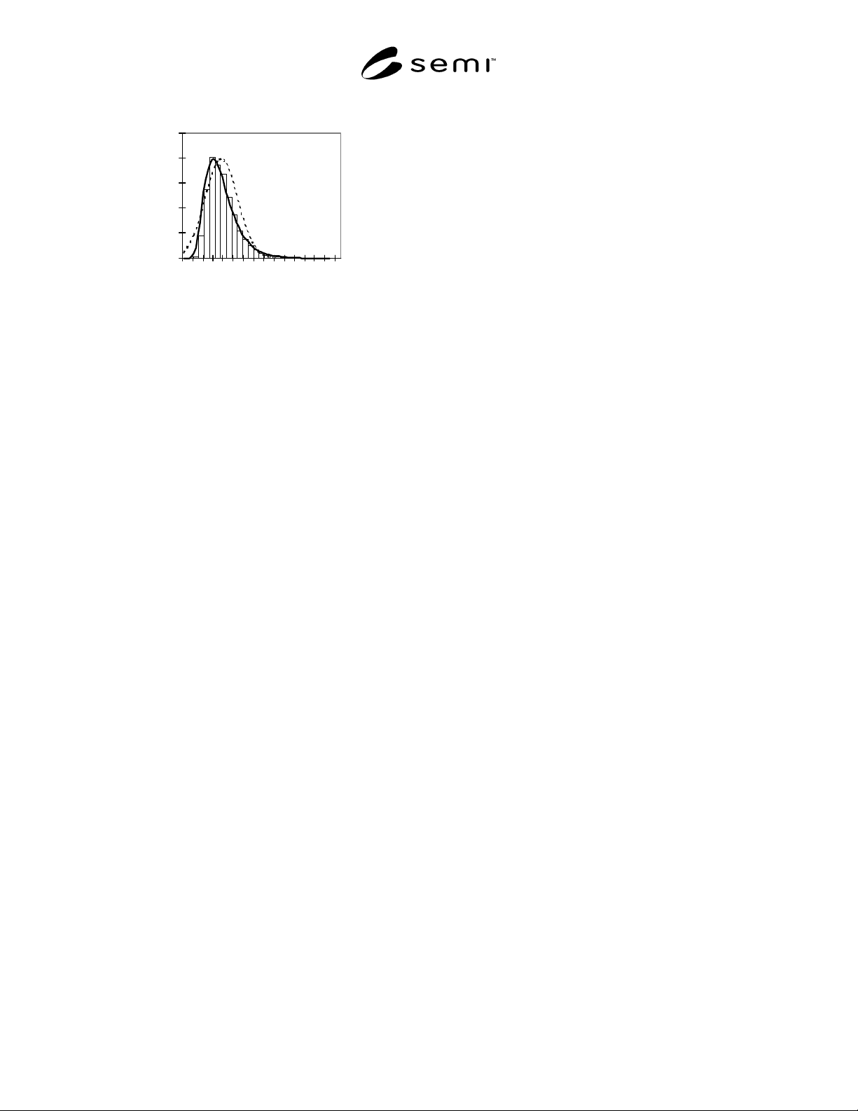
tremendous amount of knowledge. Figure A4-2 shows

an example of real data that illustrates a lognormal

process. In the past, this was considered to be difficult

because non-normal distributions were only supported

by high-level statistical software. Now even

spreadsheets have them. It should also be noted that

once the process characterization has been done, the

shape of the distribution typically does not change, so

this knowledge can be shared throughout the industry.

Regularly monitoring the process by overlaying the

distribution on the process histogram or cumulative

frequency plot is extremely valuable to confirm that the

process is not taking on unnatural bimodal or outlier

effects. One-sided distributions such as flatness and

warp are so well-characterized by the lognormal

distribution that “goodness-of-fit” results are very close

to 100%. Again, the error gets larger as the point-of

interest moves toward the “center” of the distribution,

but the major concern is the length of the tail. The

lognormal distribution in Figure A4-2 (the curve with a

solid line which is clearly not symmetrical) has a tail

that extends much farther to the right than the normal

distribution which is shown with a dashed line. This

effect, and the impact, is shown in more detail in

Appendix 2.

SEMI M32-0998 © SEMI 1998, 2004 9

500

1000

1500

2000

2500

0.0 1.0 2.0 2.9 3.9 4.8 5.8 6.7

Figure A4-2

Normal vs. Lognormal Shape

A4-1.7 Statistical specifications quantify the quality

level so it is not an abstract assumption left to

conjecture. This allows both the user and supplier to

optimize their control systems to that level. Capability

based sampling is one example. Simply put, this means

to use process capability information to help define the

sampling plan for a process. A detailed discussion of

this subject is beyond the scope of this document, but

the basic concept is easy to understand. If a process is

very capable and controlled it does not need as much

sampling as one that is not. Implementing this strategy

is a big step ahead of standard sampling theory. It might

be the only way to rigorously transfer from inspection

based quality to process control based quality, without

incurring high risks. Statistical specifications create the

environment which facilitates this improved strategy.

Hopefully, the quality levels would be defined in ppm,

but any level agreed upon by both the user and the

supplier would work.

A4-2 Tolerance Specifications

LSL to USL, or Target ± xx

A4-2.1 The main problem with a conventional

tolerance is that many people perceive it as a goal post

that requires 100% of the material to fall inside. This

document has shown in detail that this is simply a

wrong perception. Stating the quality level in the

specification, instead of just implying it, corrects this

problem.

A4-2.2 Another common misconception is that

tolerances and tail probabilities divert attention away

from centering the process. Of course, centering is

important. Considering the impact of poor quality on all

customers, it is clear that a well centered process is far

more efficient than one that is not. It is also generally

true that the suitability of the product is not

significantly different immediately on one side of a

tolerance line compared to the other. However, there

are a number of issues that warrant discussion.

A4-2.2.1 First, centering is usually not difficult, so it

usually does not need a major emphasis. Those who are

experienced in quality improvement techniques would

certainly not forget to center the process. Simply

monitoring the mean trend gives an excellent measure

of centering, and it keeps the focus on the process

rather than the specification. Industry carries a long

history where specifications prevented the attainment of

good process control. Many of the issues have been

explained earlier in this document. To summarize,

process controls are the only way to truly maintain a

centered process, and these controls can only work if

there is enough tolerance in the specification to

accommodate the sensitivity limitations of the control

methods.

A4-2.2.2 The second issue is that it might not be

possible to center. This is clearly the case in one-sided

processes that are bounded by zero. Optimizing

multiple parameters might also dictate that some

parameters get worse.

A4-2.2.3 The final, and most important, issue is the

challenge of teaching statistical methods to the factory

population. It is very easy to teach averages and

centering since they tend to be well understood already.

It is not as easy to teach sigma and the fact that sigma

trends must be thoroughly understood before much of

anything can be said about averages. Confirming that

the R or S chart is controlled before studying the Xbar

chart and doing an F-test before doing a t-test are just

two examples. These are very important concepts that

must be fully understood in order to apply statistical

methods. Over-stressing centering de-emphasizes sigma

and creates an environment where it is not appreciated.

Thinking in terms of sigma is the most important

concept that most people will learn about process

control methods. It deserves a major emphasis.

A4-2.2.4 Of course, centering would be a concern if

mixing and matching of lots is the control method, but

this can be easily spotted in the statistical

characterization process. The fact that some of the

alternatives to tolerances are much more likely to cause

this practice will be further explained in Paragraphs A4-

3 and A4-4.

A4-3 Multiple Distributional Percentile

Specifications

≤

A, %

≤

B, and % ≤ C

A4-3.1 Errors in the 10% or higher range can be

generated if a specification in the central portion of the

distribution is used. An example of such a specification

is “50% ≤ 1.2 microns”.

SEMI M32-0998 © SEMI 1998, 2004 10

A4-3.2 No control method can hold a process perfectly

still. Even the best real-time control methods can allow

a process to drift as much as ± 1.5 sigma. For this

reason, a 6-sigma design was defined as 4.5 sigma to

the nearest tolerance.

A4-3.3 Sampling issues are a major concern. Many

kinds of variation can be quantified by rigorously

studying the appropriate samplings (within batch

samples for batch-to-batch variation, monthly samples

for month-to-month variation, etc.). However, there are

practical limits on how many kinds of variation can be

continuously monitored. There is a large amount of

work involved, and there are hundreds of potential

sources of variation. Resource restrictions regularly

force suppliers to concentrate on the known key

variables and leave the rest as error in the system (at

least for now). As sample periods get longer, there is

more statistical sensitivity, but also more probability

that the drift will be confounded with user-driven

process improvements. For example, month-to-month

random drift is hard to quantify because production

processes are often improved before many months of

data can be observed. Measurement error is another

main contributor which further complicates the other

sensitivity issues. These factors all combine to allow a

certain amount of undetectable process drift. This

process drift needs to be considered when defining the

specification approach.

A4-3.4 These variations cannot be detected because of

statistical sensitivity limitations. Table A4-1 shows the

sample sizes needed to detect different levels of process

shift. Delta will be defined as the number of sigma of

undetectable mean drift. For simplicity, a one-way shift

is shown, but in most practical cases, the shift could go

plus or minus. Using the old standard of 5% supplier

risk and 10% user risk, 72 samples are needed to detect

a delta of 0.25 sigma. This example (0.25 sigma of

mean drift) has been used throughout this document.

Since most of the discussion will relate to process drift,

the terms “drift” and “shift” will be used

interchangeably. Clearly, 72 is too large a sampling for

most real-time control systems, but it is still an

understatement of the problem. Most users currently

expect their risk to be much smaller than 10%. The last

row shows that the sample size would need to be 311 to

reach 0.1% user and supplier risks. It is generally

agreed that 0.1% (i.e., 1000 ppm) is the lowest level

that is feasible using standard probability theory. For

lower levels, it is necessary to move farther out on the

distribution tails where it is necessary to rely on more

than just stndard sampling probabilities.

Table A4-1 Sampling Requirements

(a = supplier risk, b = user risk)

Detectable

Mean Shift

(in Sigma)

0.125 0.25 0.50 0.75 1.0

Min N

a = 20%

b = 20%

92 24 7 4 4

Min N

a = 5%

b = 10%

280 72 20 10 7

Min N

a = 1%

b = 1%

696 177 47 23 15

Min N

a = 0.1%

b = 0.1%

1228 311 82 40 25

A4-3.5 Figures A4-3, A4-4, and A4-5 show the error

generated by 0.25 sigma of undetectable mean drift.

Again, the number of sigma of undetectable mean drift

will be defined as delta. Notice how the error grows as

the point of interest moves toward the center of the

distribution. At the four sigma point (out on the tail)

there is very little error, so suppliers can be generous

with internal buffer specifications to protect the user.

This is not as feasible in the center of the distribution

because there is so much material at stake. A percentile

specification in the center of the process shown would

have about 1000 times more undetected, out-of-spec

product than a specification at the 4 sigma point. Since

the shift could go either way, this could also be 1000

times more material that was rejected and should not

have been.

100

8 1013151820232628

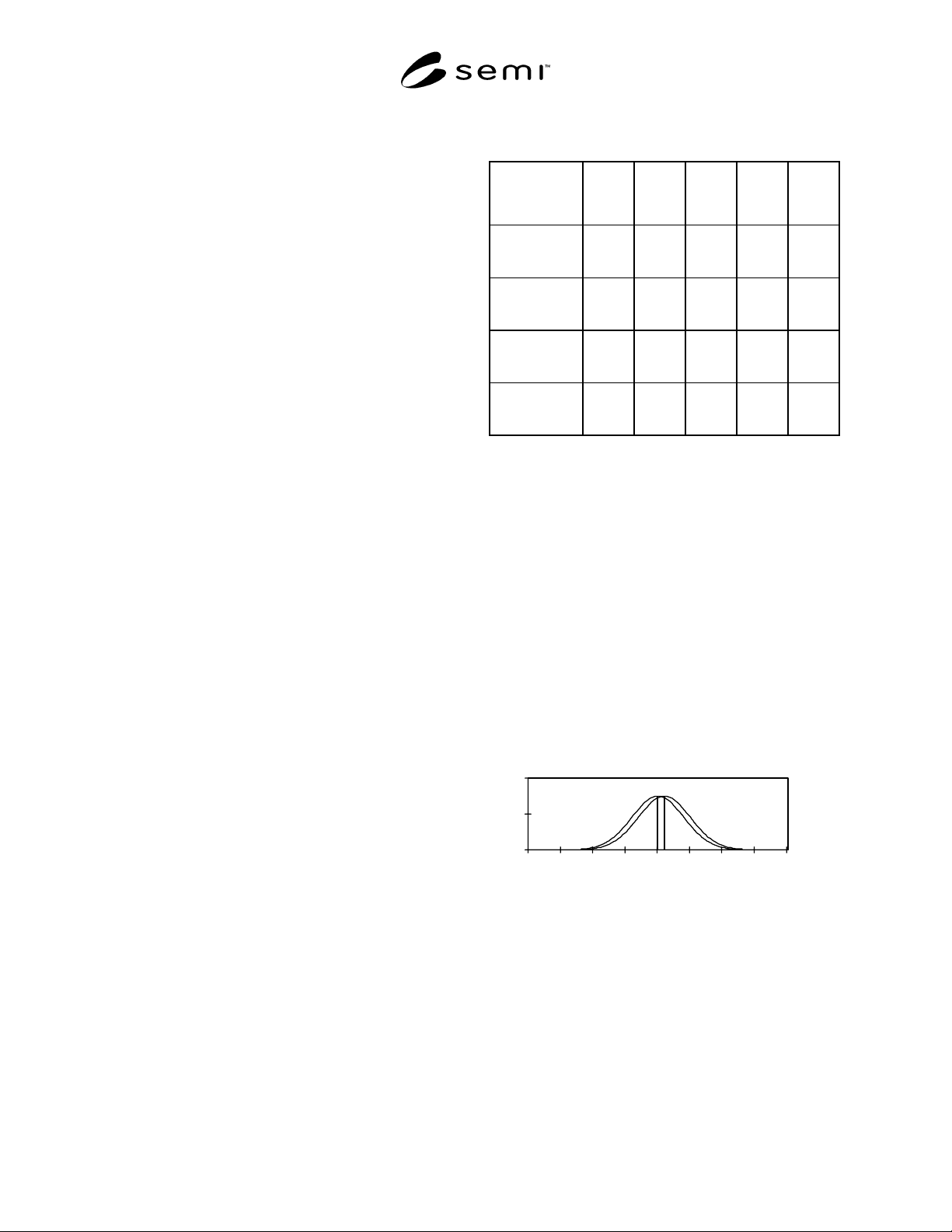
Figure A4-3

Error at 0 Sigma

A4-3.6 The left curve in Figure A4-3 shows a

distribution with an expected mean of 18. The right

curve shows the same distribution with an undetectable

drift of 0.25 sigma. If a specification limit is placed at

18, then 50% of the material is below the specification

for the nominal distribution. However, only 40.13% is

below the specification for the distribution that has

drifted. The error, shown by the area between the

vertical lines and below the right curve, is 9.87% or

98,700 ppm.