semi合集-English.pdf - 第865页

SEMI E115-0302 E © SEMI 2002 11 impedance, the m agnitude of the reflection coefficient (S11), and the magnitude of the transmission c oefficient (S21) shall be recorded. In addition, the positions of the tuning elements…

SEMI E115-0302

RELATED INFORMATION 1

LOAD SIMULATORS

NOTE: This related information is not an official part of SEMI E115 and was derived RF Diagnostic Task Force in

North America. This related information was approved for publication by full letter ballot on November 27, 2001.

R1-1 Types of Load Simulators

R1-1.1 Load Simulators are used to present a known

load impedance to a matching network. One example

of a Load Simulator would be a matching network used

in reverse. This section will describe a Load Simulator

that can be used with typical matching networks that

operate at 13.56 MHz with capacitive load impedances.

These applications include those networks used in

parallel-plate capacitively coupled plasmas and also

those networks used in wafer bias applications, where

the plasma is mostly sustained by another power

source, such as an inductively coupled plasma or a

microwave ECR (electron cyclotron resonance) plasma.

R1-1.2 The typical impedance that is seen by the

matching network depends on the geometry of the

applicator (its capacitance to ground), the type of

plasma (gases), the operating pressure, and the density

of the plasma. Typical impedances seen by the

matching networks operating at 13.56 MHz in

capacitive-loading applications have a real part in the

range of 0.5 to 10 ohms and a reactive part in the range

of –10 to –50 ohms. If a transmission line is used

between the output of the matching network and the

applicator, the impedance will get transformed. The

amount of transformation will depend on the length of

the transmission line, but in general the effect will be to

decrease the real part of the impedance and to decrease

the reactive part of the load (make it less negative). If

the transmission line is long enough, the impedance

seen by the matching network may even look inductive

instead of capacitive because of the impedance

transformation.

R1-2 Load Simulator Design

R1-2.1 A typical design for a Load Simulator operated

at 13.56 MHz uses two capacitors and a 50-ohm load.

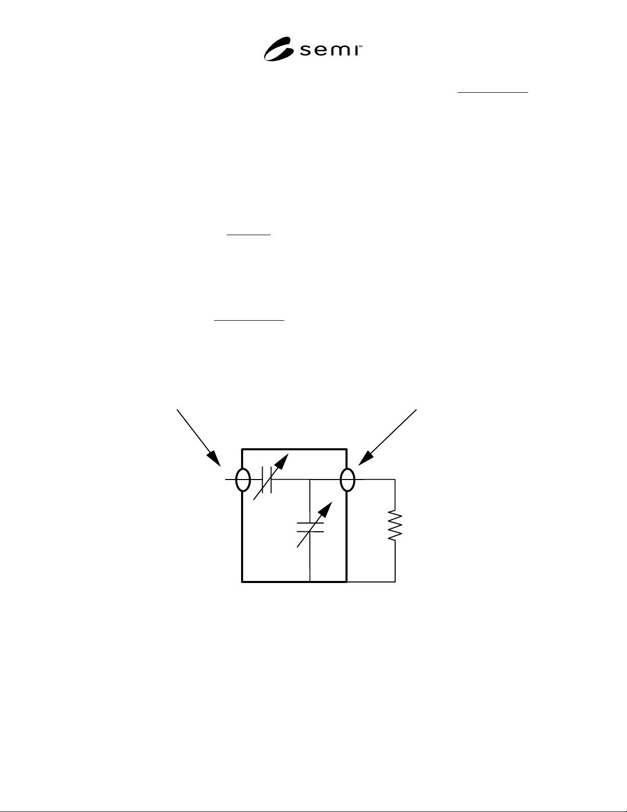
A schematic is shown in Figure R1-1. The Load

Simulator consists of a series capacitor, C2, and a shunt

capacitor, C1. The C1 capacitor is in parallel with a 50-

ohm load. The 50-ohm load can be an input port to a

Network Analyzer or a high-power 50-ohm load that

can be used with high-power testing.

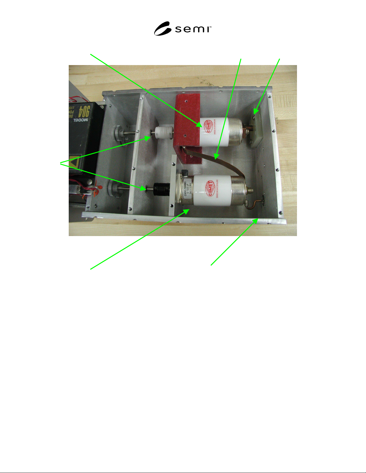
R1-2.2 A picture of a Load Simulator of this type of

design is shown in Figure R1-2. Two vacuum variable

capacitors are used, with a copper strap connecting

them. The capacitors shown in the figure are variable

from 8 to 1000 pF. Additional fixed capacitors can be

easily added to the circuit to expand the operating

range. The strap connecting the capacitors adds

roughly 100 nH of inductance to the series part of the

circuit for this example.

R1-2.3 The impedance range for this type of Load

Simulator is fairly broad. A plot of the real part of the

input impedance as a function of the value of the C1

shunt capacitor is shown in Figure R1-3. The real part

of the load varies from close to 50 ohms to around 1.2

ohms at a C1 capacitance of 1500 pF. A plot of the

reactive part of the input impedance is shown in Figure

R1-4. The reactance can be varied as a function of both

the C1 and C2 capacitances. A reactance range of –5 to

–100 ohms is easily achieved for a C2 capacitance

variation of 1500 pF to 100 pF.

R1-3 Measurement of Load Simulator

Impedance and Efficiency

R1-3.1 The impedance and the efficiency of the Load

Simulator can be measured in much the same way as a

matching network. The test setup is shown in Figure R-

5. A special fixture may be required to adapt the input

connection of the Load Simulator to a coaxial

connector.

R1-3.2 Calibrate the Network Analyzer at the desired

operating frequency (e.g., 13.56 MHz). The Network

Analyzer shall be calibrated for measuring the

reflection coefficient at test Port 1 and for measuring

the transmission coefficient at test Port 2 (see Figure R-

1) using the calibration kit provided with the Network

Analyzer. This measurement requires measuring the

S11 and S21 S-parameters and requires a full 2-port

calibration. The calibration shall be performed at fixed

frequency (continuous-wave operation) using the

lowest bandwidth possible (typically 10 Hz). The

calibration for each port shall include the additional test

cables and any additional adapters.

R1-3.3 After calibration of the Network Analyzer, the

cable connected to Port 1 of the Network Analyzer shall

be connected to the input of the Load Simulator. The

cable connected to Port 2 of the Network Analyzer shall

be connected to the output of the Load Simulator.

R1-3.4 The tuning elements (variable capacitors) shall

be moved to their minimum positions before the

measurement is initiated. After all connections are

visually inspected for proper contact and the Network

Analyzer has stabilized, the value of the input

SEMI E115-0302

impedance, the magnitude of the reflection coefficient

(S11), and the magnitude of the transmission coefficient

(S21) shall be recorded. In addition, the positions of

the tuning elements of the Load Simulator shall be

recorded.

R1-3.5 The efficiency of the Load Simulator is

determined from both the reflection and transmission

coefficients. The efficiency can be calculated by taking

the ratio of the output power divided by the input

power. The output power is simply (S21)

and the

input power is (1-(S11)

()

111

iencyator EfficLoad Simul

−

Typically, the reflection and transmission coefficients

are expressed in terms of dB (decibels). The conversion

between dB and efficiency is expressed as

)10/dBin 11S(

)10/dBin 21S(

101

−

=EfficiencySimulator Load

)10/dBin 11S(

)10/dBin 21S(

101

100%

−

×=TransferPower

For example, if the transmission coefficient is measured

to be –10 dB and the reflection coefficient is measured

to be –0.5 dB, then the power transfer efficiency would

be 91.95%. In other words, 8.05% of the power is lost

in the Load Simulator.

R1-3.6 For the next measurement, one tuning element

shall remain fixed (C2), and the other tuning element

(C1) shall be increased by an increment equal to no

more than 10% of the full scale range of the tuning

element position. After the tuning elements have been

moved to their new values, steps 3.4 and 3.5 shall be

repeated. This process shall be repeated until the tuning

element (C1) has covered its entire range.

R1-3.7 After the tuning element (C1) has been varied

over its entire range, the other tuning element (C2) shall

be increased by an increment equal to no more than

10% of its full-scale range. The C1 tuning element

shall then be moved back to its minimum position and

the above steps (R1.3.4–R1.3.6) shall be repeated until

the entire tuning range of the matching network is

measured.

Load Simulator

Input Connection

Output Connection

50-Ohm Load

NOTE 1: The input connection is attached to a series variable capacitor, C2. The shunt variable capacitor, C1, is in parallel with

a 50-ohm load.

Figure R1-1

Schematic of a Load Simulator

SEMI E115-0302

Series Capacitor Strap Input

Rotating

Shafts

Shunt Capacitor Output

NOTE 1: Picture of a Load Simulator showing the variable capacitors. The capacitors are connected together by a strap that has

an inductance of around 100 nH. The values of the capacitors are varied by rotating their shafts. The ends of the shafts are

connected to a dial indicator to measure their positions.

Figure R1-2

Picture of a Load Simulator Showing the Variable Capacitors