semi合集-English.pdf - 第5165页

SEMI M32-0998 © SEMI 1998, 2004 4 A1-3.4 Once a process has been statistically characterized, everything becom es much easier. Calculati ons can be do ne in milliseconds inst ead of minutes. This includes spec acceptance…

SEMI M32-0998 © SEMI 1998, 2004 3

APPENDIX 1

USING STATISTICAL SPECIFICATIONS FOR NORMAL PROCESSES

NOTICE: This appendix was approved as an official part of SEMI M32 by full letter ballot procedure.

A1-1 Statistical Specification Format for

Normal Distributions

A1-1.1 The normal distribution is quite well-known. It

describes processes that target a specific value and have

symmetric random variation about that value. Below

are examples of statistical specifications for normal

processes. The first portion is the familiar tolerance,

and the second portion is a measure of the quality level.

LSL to USL @ yy ppm, o

Target ± xx @ yy ppm

Other standard tolerance definitions could be

substituted, or other definitions of the quality level such

as Cpk, Z-value, or percent could be used.

A1-1.2 Adding the quality level removes the potential

for misunderstanding and makes the specification more

meaningful.

A1-2 Example of Use

A1-2.1 Functionally, statistical specifications are

similar to conventional tolerances, except that the

quality level is stated rather than just implied. They can

be directly substituted for tolerances or other forms of

specifications. Statistical specifications are especially

useful for focusing quality improvement efforts,

achieving ship-to-stock relationships, promoting

processed in quality, and reducing after the fact

inspection. In this environment they could be used as

follows:

A1-2.1.1 Through audits and capability reporting a

particular parameter is targeted for improvement or

chosen as a ship-to-stock candidate.

A1-2.1.2 The control methods, distribution shape, and

statistical specification are agreed upon. The tolerance

and quality level defined in the statistical specification

completely define the needed process capability.

A1-2.1.3 Once it is shown that the required capability

is consistently exceeded then reduced inspection

sampling can be implemented without increasing the

risk to the customer or supplier. In this way the process

controls can gradually become the guarantee for

quality, and after the fact inspection can be gradually

reduced to the level that is needed for outgoing quality

reporting.

A1-3 Discussion

A1-3.1 Statistical specifications remove ambiguity,

allow small risks, and promote the movement toward

better process controls and less after the fact inspection.

The quality level (i.e., the yy portion) is often

misunderstood. Some people say they want ppm level

quality but introduce methods that allow 50,000 to

200,000 ppm in error. This causes confusion.

A1-3.2 Many people have the misconception that

tolerances are goal posts that require 100% of the

material to fall inside. Processes are usually described

by statistical distributions, so specifications have little

meaning if a quality level is not defined. For many

years, 99.73% (i.e., ± 3 sigma) was considered to be

satisfactory. “Within tolerance” was understood to

mean within tolerance with a 99.73% confidence, or a

0.27% quality level. Later the 99.73% process was

defined as “cruel”. 0.27% was no longer an acceptable

quality level, and process drift was understood to cause

even higher reject rates. This led to the demand for

better process capabilities (i.e., higher Cpk’s), which

demanded corresponding improvements in process

characterization and control methodologies. At the

same time other users tightened their tolerances to the

point that led to over-control. Either extreme can cause

a mismatch between expectations and capabilities if the

risks are not carefully evaluated.

A1-3.3 Capability-based sampling is perhaps the only

way to rigorously transfer from inspection-based

quality to process control-based quality, without

incurring high risks. Statistical specifications create the

environment for this to work. Once the specification is

clearly defined, it can be clearly achieved. The details

of capability based sampling are beyond the scope of

this document, but the basic concept is easy to

understand. If a process is very capable and controlled,

then the system can be relied upon to create the

necessary quality level with less after the fact

inspection. This is good for both sides. Users get more

reliable quality, and suppliers get the information

needed to focus quality improvement efforts and direct

resources at the most critical processes.

SEMI M32-0998 © SEMI 1998, 2004 4

A1-3.4 Once a process has been statistically

characterized, everything becomes much easier.

Calculations can be done in milliseconds instead of

minutes. This includes spec acceptance, comparisons,

and many forms of analysis. Multiple levels like % < A,

% < B, and % < C are also clearly unnecessary if the

distribution shape is known. This prevents a large

amount of duplicate work.

SEMI M32-0998 © SEMI 1998, 2004 5

APPENDIX 2

USING STATISTICAL SPECIFICATIONS FOR LOGNORMAL

PROCESSES

NOTICE: This appendix was approved as an official part of SEMI M32 by full letter ballot procedure.

A2-1 Statistical Specification Format for

Lognormal Distributions

A2-1.1 The lognormal probability distribution function

describes many of the one-sided distributions

encountered in the silicon industry. It applies to those

one-sided parameters like flatness and warp that are

bounded by zero. Below is an example of a statistical

specification for a lognormal process.

≤ xx @ yy ppm

A2-1.2 Other standard tolerance definitions could be

substituted, or other quality level definitions such as

ECPK, Z-value, or percent could be used. Again, ECPK

is the Equivalent normal Cpk that corrects for non-

normality. More information on the Equivalent Cpk is

shown at the end of this appendix.

A2-1.3 As with the normal distribution, adding the

quality level removes the potential for

misunderstanding and makes the specification more

meaningful.

A2-2 Example of Use

A2-2.1 Again, the major objectives are to focus quality

improvement efforts, achieve ship-to-stock

relationships, promote processed in quality, and reduce

after the fact inspection. The steps are the same as

shown in Section A1-2 for the normal distribution. The

major difference is that only the upper tail needs to be

considered. However, since the lognormal tail goes so

much farther out, it might be necessary to accept a less

critical quality level.

A2-3 Discussion

A2-3.1 Statistical specifications work very well for

processes with lognormal distributions. They have all

the benefits described for normal distributions, and in

some respects, they are even easier. Since lognormal

processes only have one tail, checking each tail to

decide which is the most critical is not necessary. Also,

it has been empirically observed that lognormal

processes are not as prone to mean drifting, so they tend

to be more stable. The main hurdle is realizing how

much error is introduced if the distribution shape is

assumed to be normal when it is not.

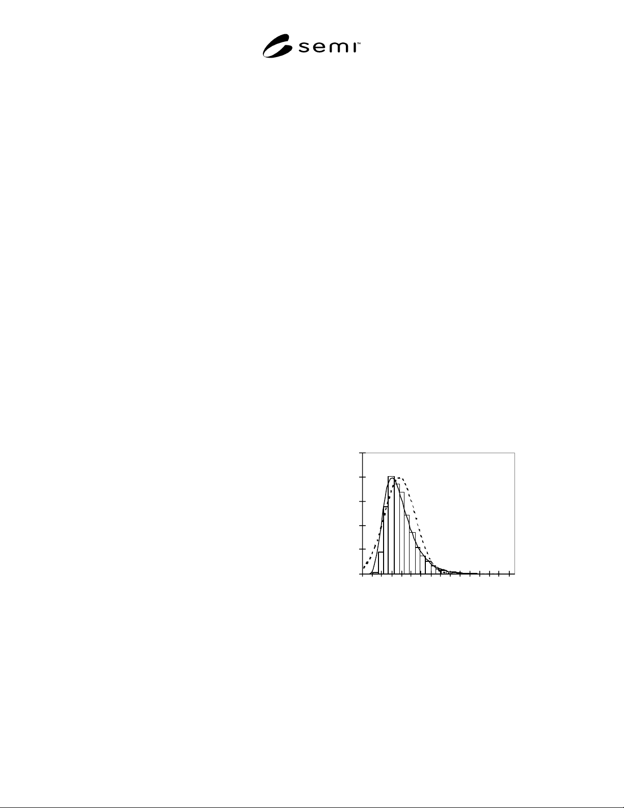
A2-3.1.1 Figure A2-1 illustrates the difference between

a lognormal and a normal process. The curve which has

a solid line (and is clearly not symmetrical) is the

lognormal distribution. The curve with the dashed line

is the normal distribution. The error when mistakenly

using a normal distribution to characterize a lognormal

process is shown in Table A2-1. For values that

increment by 1 sigma from the mean, the ppm greater

than that value is given for each curve, and the

difference (or error) is calculated. To make it easier to

visualize, increments of the simple normal mean and

sigma (1.8263 and 0.7568 respectively) are used in the

“value” column. For calculating the lognormal statistics

the correct lognormal geometric mean of 1.8258 and

the lognormal geometric sigma of 0.7550 are used. The

error between the curves increases as the point of

interest moves toward the center of the distribution, but

the most important issue is the length of the tail. The

right tail of the lognormal distribution extends along

with the histogram, but the normal distribution is much

shorter. Visually, the significance might be overlooked

in Figure A2-1, but when the tail probabilities are

shown in ppm (Table A2-1) the difference is very

apparent.

500

1000

1500

2000

2500

0.0 1.0 2.0 2.9 3.9 4.8 5.8 6.7

Figure A2-1

Lognormal vs. Normal Curves