semi合集-English.pdf - 第688页

SEMI E89-1104 E © SEMI 1999, 2004 15 R3-2.6 When error terms are known to have nonnormal distributions, special methods and/or software (beyo nd the scope of this guide) are needed. NOTE 1: The model might als o include …

SEMI E89-1104

RELATED INFORMATION 3

MODELS FOR MEASUREMENT SYSTEM ANALYSIS

NOTICE: This related information is not an official part of SEMI E89. It was derived from task force deliberations

during the revision of SEMI E89-0999 in 2001-2003. This related information was approved by full letter ballot

procedures and was approved for publication by the NA RSC on August 16, 2004.

R3-1 Introduction

R3-1.1 This related information section provides a

more detailed theoretical explanation that extends ideas

described earlier in this guide.

R3-1.2 A measurement model expresses each observed

measurement value as the sum of a “true value” plus

“bias” plus “random error.” The “true value” may be

the actual value for the object being measured or the

average population value if a sample of objects is

measured in the MSA. The random error term is

further broken up into contributions from all the

significant sources of error under investigation. If an

MSA is well designed, standard statistical techniques

(such as ANOVA) can be used to estimate the standard

deviation contribution from each source of error, and

from this the repeatability, reproducibility and precision

of the MS are determined.

R3-1.3

Note that any MS that is composed of several

measurement subsystems (such as spectrometry and

ellipsometry), designed for the measurement of

different characteristics or types of samples, should be

treated as composed of separate MSs that need to be

analyzed independently.

R3-1.4

Writing an appropriate measurement model is

the starting point, after which many software packages

can be used to design the MSA and calculate ANOVA

estimates from the resulting measurement data.

R3-1.4.1

The model must indicate whether each source

of variation, i.e., factor, is fixed or random. Variance

components are only available for random factors.

R3-1.4.2 The model must indicate which factors are

crossed and which are nested.

R3-2 Example of a Measurement Model

R3-2.1 A wafer oxide thickness MS is under

investigation. A wafer is placed in the gauge, which

then automatically positions the wafer and takes a

measurement. While the wafer is positioned, the

measurement can be repeated as many times as desired.

Sources of variability that might affect a measurement

include basic repeatability on a positioned wafer,

variability due to the automatic positioning process,

variability over time and variability from measuring

several different wafers (to cover a range of “true”

measurement values).

R3-2.2

An MSA that separates out all these possible

sources of variability is the following: 10 wafers are

chosen at random from normal production. Each wafer

is put in the MS in a random order and measured 3

times at a single site (3 repeats) on day 1 (cycle 1).

Immediately after the 30 measurements are recorded,

the same measurement process is repeated on the 10

wafers (cycle 2). On day 2, the same wafers are again

measured using exactly the same procedure. This is

repeated for a total of 5 days, yielding 3 × 10 × 2 × 5 =

300 measurements.

R3-2.3

Assuming the MS has been calibrated (or bias

is not a concern at the moment), a model for variability

is constructed as follows: let h = 1, 2, …, 5, index the

days; let k = 1, 2, …, 10, index the wafers; let j = 1, 2,

index the repositions (cycles) each day and let i = 1, 2,

3, index the repeat measurements (taken under

repeatability conditions) on a positioned wafer.

R3-2.4 The model for the i

measurement at the j

repositioning on the k

wafer on the h

day is:

hkji



+ d

+ w

+ p

hkj

+ r

hkji

(R3-1)

where:

hkji

= measurement taken on day h, wafer k, cycle j,

and repeat i,



= true oxide thickness average value for the

population of wafers,

= error term associated with the h

day (due to

day-to-day stability variation),

= offset from the average due to the true

thickness of the film on wafer k,

hkj

= (short term) error due to the j

positioning of

the k

wafer on the h

day, and

hkji

= repeatability error term.

R3-2.5 In this model, the quantities d

, p

hkj

, and r

hkji

are

random error terms. They are usually assumed to have

a normal distribution with zero mean and standard

deviations



, and



, respectively. The wafer term

may be either a random term or a “fixed effect,”

depending on whether we consider the wafers measured

to be a random sample from the entire population of

possible wafers or a fixed population used for

experimental purposes. In either case, the estimates of

repeatability and reproducibility will be the same.

SEMI E89-1104

R3-2.6 When error terms are known to have

nonnormal distributions, special methods and/or

software (beyond the scope of this guide) are needed.

NOTE 1: The model might also include a wafer-by-day

random error term wd

hki

, if it is suspected that measurements

made from day to day on some wafers might vary differently

than measurements made from day to day on other wafers,

and it is desired to obtain an estimate of this component of

reproducibility.

R3-2.7 Reproducibility includes everything but wafer-

to-wafer true thickness variability, so

222

rpdR



 (R3-2)

R3-2.8

The ANOVA for this MSA provides all the

variance estimates needed to calculate repeatability,

reproducibility and precision. If the wafer term w

random, the ANOVA will also estimate



, which is

useful for characterizing the wafer population

variability.

NOTE 2: When inputting this model into a statistical analysis

program, the factors “day” and “wafer” are said to be crossed,

since every wafer is measured on every day. The factor

“positioning” is nested within wafer and day, and

“repeatability” is the residual error term and is nested within

positioning, wafer and day. A factor “A” is nested within

another factor “B” if the levels or values of “A” are different

for every level or value of “B.”

R3-2.9 This example shows how a fairly complicated

MSA can be set up. Each particular situation can lead

to a different model and experimental design,

depending upon the goals and agreed upon sources of

(possibly significant) variation.

SEMI E89-1104

RELATED INFORMATION 4

EXAMPLE OF A MEASUREMENT SYSTEM ANALYSIS

NOTICE: This related information is not an official part of SEMI E89. It was derived from task force deliberations

during the revision of SEMI E89-0999 in 2001-2003. This related information was approved by full letter ballot

procedures and was approved for publication by the NA RSC on August 16, 2004.

R4-1 Introduction

R4-1.1 The following example illustrates how an MSA

was performed on an automated wafer film thickness

MS for the purpose of determining the reproducibility

and variance components. The MS was calibrated prior

to the MSA, but the presence of bias would not affect

the estimation of variance components as long as the

amount of bias does not change over the course of the

MSA. Different wafer types were selected to span the

range of both possible wafer types and typical

thicknesses. Five standard wafers were manufactured

with characteristics as shown in Table R4-1.

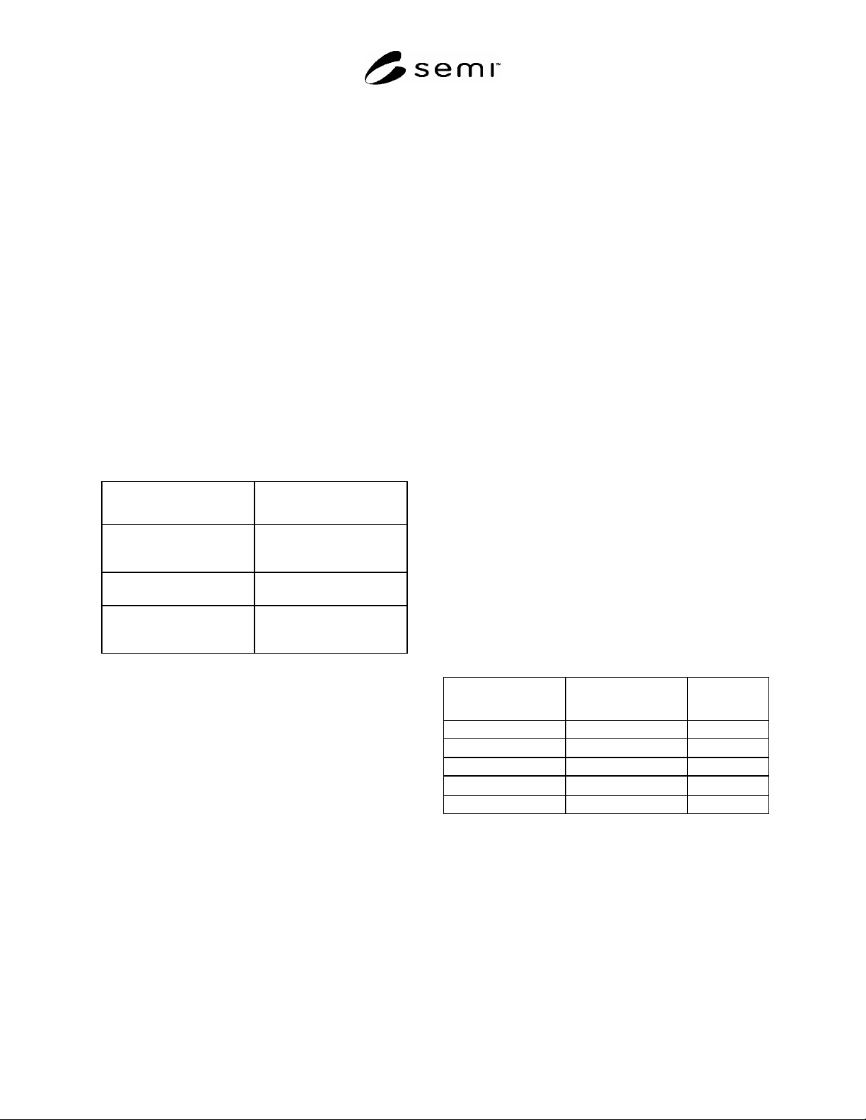
Table R4-1 Wafers Used for Analysis

Film Type

Total Nominal Film

Thickness (Å)

Oxide (wafers 1, 2, 3) 50, 980, 7900

(for wafers 1, 2, 3,

respectively)

Polysilicon over Oxide

(wafer 4)

2,575

Deep UV Resist over

ARC over Oxide

(wafer 5)

13,000

UV  Ultra Violet, ARC  Anti Reflective Coating.

R4-1.2 Wafers were measured on eight days, evenly

spaced over a two-week period. On each day of the

MSA each wafer was chosen twice, loaded each time

into the gauge and measured twice without unloading.

The order of selection was random. Therefore, on a

given day, each wafer was measured exactly four times.

Measurements were taken at three points on the wafers

and averaged. The model (see Related Information 3)

used was

hkji



+ d

+ w

+ wd

+ c

hkj

+ r

hkji

+ e

hij

(R4-1)

where:

hkji

= measurement result (average of measurements

taken at three points each time) on day h,

wafer k, cycle j, and repeat i,



= grand mean of film thickness value across all

conditions,

= effect or contribution associated with the h

day (due to day-to-day stability variation),

= offset from the average due to the true

thickness of the film on wafer k,

= effect or contribution due to wafer-by-day

(wafer  day) interaction,

hkj

= effect or contribution due to cycle j, nested in

wafer k and day h,

hkji

= effect or contribution due to repeat i, nested in

cycle j, wafer k, and day h, and

hij

= residual effect due to all terms not included in

the model.

R4-1.2.1 The variabilities contributed by d

, wd

, and

hkj

are part of reproducibility. The variability

contributed by r

hkji

is the repeatability.

R4-2 Analysis

R4-2.1 Most statistical analysis software programs

report estimates as variances and produce the variance

components analysis shown in Table R4-2. (Methods

of moments estimates were used. Negative variance

components were set to zero). Sources of variation,

such as



and



, are standard deviations found by

taking the square roots of the appropriate variance

component or sum of components.

Table R4-2 Variance Components Estimates — All 5

Wafers

Variance

Component

Estimated

Variance

Estimated

Sigma

Day 12.1348 3.4835

Cycle 0.1256 0.3544

Repeat 0 0.0000

Wafer  Day

462.9869 21.5171

Residual 0.8446 0.9190

R4-2.2 Wafer variability (



wafer

) was not reported

because it is associated with a fixed effect. Variance

components are only estimated for random effects. If,

for example, the five wafers were randomly selected

from a distribution for a single wafer type, wafer

variability would be included in the table and could be

used to estimate the SNR. However, wafer variability

would still not be part of



. For further details, see

Related Information 3.