semi合集-English.pdf - 第956页
SEMI E124-1103 © SEMI 2003 11 R1-1.6 We can now see why the efficiency of throughput rate and cycle time can both be measured by the same metric ( throughput-rate and cycle-time efficiency ). The following derivation als…
SEMI E124-1103 © SEMI 2003 10
R1-1.5 Now suppose the factory is managed with a
pull strategy where a constant WIP level is enforced so
that throughput rates are allowed to reach their
equilibrium state. In general, this is a better strategy,
because studies have shown that a constant WIP level
will result in a higher average throughput rate than the
constant throughput rate that results in the same average
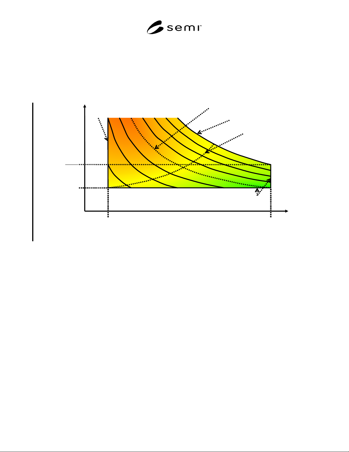
WIP level. As shown below in Figure R1-4, this
constant WIP strategy (known as CONWIP) amounts to
choosing to operate the factory on one of the solid black
curves (each of which represents a different constant
WIP level). We try to drive the factory along that curve
toward the bottom right (for lower average cycle time
and a higher actual throughput rate) by using better
operating principles, but we are resisted by the inherent
variability of the factory.
actual throughput rate
1/T
min
bottleneck
throughput
rate (R
max
)
Threshold Case
(normalized
production
efficiency = ½)
critical WIP (W
0
= R
max
×T
min
)
WIP capacity (W
max
)
Best Case (throughput-rate & cycle-time efficiency = 1)
average
cycle time
theo-
retical
cycle
time
(T
min
)
W
max
R
max
Worst Case (throughput-rate
& cycle-time efficiency = 1/W
0
)
G
r
e
e
n
Yellow
Red
Figure R1-4
Plot of Average Cycle Time vs. Actual Throughput Rate

SEMI E124-1103 © SEMI 2003 11
R1-1.6 We can now see why the efficiency of
throughput rate and cycle time can both be measured by
the same metric (throughput-rate and cycle-time
efficiency). The following derivation also gives
alternative definitions for throughput-rate and cycle-
time efficiency for use when cycle time information is
not available (such as in resource-based simulations).
(
)
-
-
throughput rate and
cycle time efficiency
()
()
()
max ,
max ,
-
average WIP
theoretical
cycle time
bottleneck throughput rate
average cycle time
average
WIP
theoretical
cycle ti
best case cycle time
average cycle
me
bottleneck
throughput
rat
time
e
=
=
=
()
()()
()
()
1
max ,
1
min
average
WIP
average average
cycle time WIP
theoretical cycle time
bottleneck
average WIP
throughput rate
actual throughput rate
actual throughput rate
average WIP
theoretical cycle
=
=
()
()()
()( )
,
-
bottleneck
throughput rate
time
finished units out total time
average WIP theoretical cycle time
act
theoretical cycle time finished units out
ual throughput
total ti
rate
best case throughput rat
m
e
ea
=
=
=×
()()
as a fraction of
verage WIP
theoretical cycle time WIP
total time turnover
=×
(2)
R1-1.7 The production efficiency is normalized by the
power of the normalizing exponent so that a value of ½
for the normalized production efficiency indicates that
the factory is performing at the level of the threshold
case (which divides a well run factory from one badly
operated). This threshold case is also known as the
practical worst case, because it represents what the best
operating procedures can do in a maximally random
factory (see the Factory Physics book for more on this
case). In the threshold case,
()
(
)
(
)
1
average critical
WIP WIP
average
cycle time
bottleneck throughput rate
+−
= (3)
which results in the following production efficiency.
(
)
production
efficiency
(
)
(
)
()
()
()
()
-
-
max ,
max
throughput rate and WIP
cycle time efficiency efficiency
average
WIP
theoretical
cycle time
bottleneck
throughput
rate
WIP
efficiency
average cycle time
bo
theoretical
cycle time
=×
=×
×
=
()
()( )
()
()( )
{}
,
max ,
ttleneck
average
throughput
WIP
rate
average bottleneck
cycle time throughput rate
WIP efficiency
critical average
WIP WIP
×
×
=
()( )
{}
()( )
{}
min ,
max ,
average bottleneck
cycle throughput
time rate
critical average
WIP WIP
critical average
WIP WIP
×
×
()( )
{}
()()
()
min ,
1
critical average
WIP WIP
average critical
WIP WIP
bottleneck
throughput rate
=
+−
bottleneck
throughput
rate
×
()()
{}
()()
min ,
1
average critical
WIP WIP
average WIP critical WIP
=
+−
(4)

SEMI E124-1103 © SEMI 2003 12
R1-1.8 Thus, if we set normalized production
efficiency to have a value of ½ at this average cycle
time, we get
()
()
()()
{}
()()
()
1
2
min ,
1
normalizing
exponent
normalizing
exponent
normalized
production
efficiency
production
efficiency
average critical
WIP WIP
average critical
WIP WIP
=
=
=
+−
(5)
and, taking logarithms of both sides,
2
1
log
2
()()
{}
()()
()
()()
{}
()()
2
2
min ,
log
1
min ,
log
1
normalizing
exponent
average critical
WIP WIP
average critical
WIP WIP
average critical
WIP WIP
normalizing
exponent
average critical
WIP WIP
=
+−
=×
+−
(6)
so
()
()()
{}
()()
()()
()()
{}
()()
2
2
2
2
1
log
2
min ,
log
1
1
1
log
min ,
1
log
normalizing
exponent
average critical
WIP WIP
average critical
WIP WIP
average critical
WIP WIP
average critical
WIP WIP
average critical
WIP WIP
=
+−
−
=
+−
−
=
+
()()
{}
1
min ,
average critical
WIP WIP
−
(1)
which is the same as Equation (9) that was given in
Section 6 of the main body of this guide.