semi合集-English.pdf - 第586页

SEMI E79-0304 © SEMI 1999, 2004 20 Pre-Align Load Set & Align Load Box Reticle Handler Pre-Al ign Chuck x (# wafers per reticle) Exposu re Sta ge 1.1 Expose Transfer Tr ansf er Pre- Align Load Figure R1-1 Example Res…

SEMI E79-0304 © SEMI 1999, 2004 19

group of elements defined elsewhere. This group is

referred to as a sub-sequence.

1.1 Sub-Sequence

Operational Element

R1-2.6 Calculating Theoretical Production Time Per

Unit — Any element sequence may be modeled as an

activity-on-node network derived from precedence

constraints on the operational elements and precedence

constraints on the allocation of equipment resources to

the elements. Using the network model, the duration of

the element sequence is simply the duration of the

critical path through the network.

R1-2.6.1 Theoretical production time per unit is then

the theoretical duration for the element sequence

divided by the number of units processed during the

sequence.

Theoretical Production Time Per Unit for recipe i [THT

= (Theoretical Duration for the Element Sequence)

/(Number of Units Processed During Sequence)

R1-2.7 Allowances for Non-Steady-State Processing —

For complicated batch-load equipment models, it is

useful to divide resource sequences into a beginning

phase, a steady-state-phase, and an ending phase. For

modeling theoretical time, it is important to determine

what allowances to make, if any, for the beginning and

ending phases. For machines that are limited in the

number of lots that can be processed in a continuous

cascade, appropriate allowances shall be made for

beginning and ending phases. However, for machines

that are capable of running continuously, the beginning

and ending phases should not be considered in

determining theoretical production time.

R1-2.7.1 Under certain conditions, setup type

operations that are not tracked as part of downtime shall

be considered as part of the theoretical resource

sequence for a tool. These conditions include

operations that shall occur in every machine cycle, e.g.

recipe download, as well as operations that occur on

other regular intervals, e.g., one clean cycle every 75

wafers. In general, any activity that occurs on

predictable intervals and is a necessary part of a recipe

specification should be considered in the equipment

sequence for determining theoretical production time.

R1-2.7.2 Operations that occur at irregular intervals or

that apply to an unpredictable quantity of wafers, lots,

or loads are not counted. An example of an

unpredictable frequency setup is a recipe changeover,

when the machine is changed from the requirements of

one process recipe to meet the needs of another, e.g., a

species change as on an ion implant system. The ideal

frequency of these events is taken as zero.

R1-2.8 Optimality — Theoretical sequences shall be

designed so as to optimize equipment throughput by

using only the best configuration of elements and an

optimal load size. Optimal sequences may differ for

different recipes performed on the same machine.

Optimal load sizes are not necessarily maximum load

sizes.

R1-2.9 Error-Checking Element Sequences  Once a

theoretical sequence is specified for a piece of

equipment, it can be compared against actual equipment

operations to check for errors. If discrepancies are

found, three possibilities to investigate are:

• The sequence contains extraneous elements.

• The sequence is missing necessary elements.

• The series and parallel relationships between

elements are not correctly specified.

R1-2.9.1 What may at first appear to be sequence

specification errors may in fact be undiscovered rate

efficiency losses embedded in the equipment sequence.

Because sequences are fundamental to overall

performance, it is important to rule out sequence

specification errors to preclude erroneous assignment of

rate efficiency losses to individual elements.

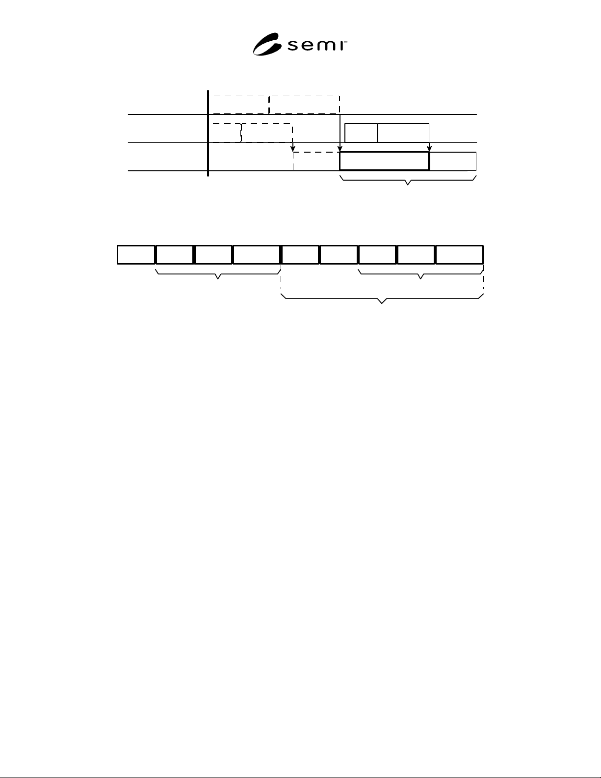
R1-2.10 Example Resource Utilization Sequence  An

example of a resource utilization sequence is given in

Figure R1-1. This example represents a particular

instance of a photolithography stepper that exposes

patterns from a reticle onto a wafer. This example

assumes that the stepper receives individual unexposed

wafers from a linked coat track and transfers individual

exposed wafers to a linked develop track.

R1-2.10.1 First, a reticle box shall be loaded into the

stepper reticle handling system (“load box”). Before a

wafer may be exposed, the reticle shall be set and

aligned. A wafer shall also be loaded onto the pre-align

chuck, pre-aligned, and transferred to the exposure

stage. Each wafer is exposed then transferred to a post

processing relay chuck. The transfer operation

simultaneously removes an exposed wafer and replaces

it with an unexposed wafer.

R1-2.10.2 The expose operation is represented by the

sub-sequence shown in Figure R1-2. Depending on the

recipe to be executed, the expose sub-sequence may

consist of several different reticle images requiring

changes of “blade” positioning. For each image, there is

one “align” operation. For each individual exposure,

there is a “step” operation, a “level” operation, and the

“expose” operation itself. Within the same image,

different exposures may require different leveling

times, as well as different stepping times.

SEMI E79-0304 © SEMI 1999, 2004 20

Pre-AlignLoad

Set & Align

Load Box

Reticle Handler

Pre-Align Chuck

x (# wafers per reticle)

Exposure Stage

1.1 ExposeTransfer Transfer

Pre-AlignLoad

Figure R1-1

Example Resource Utilization Sequence

Step

Align Level Expose

x (# exposures)

Blade

Align

x (# exposures)

x (# images-1)

Step Level Expose

Figure R1-2

Example of Equipment Sub-Sequence

R1-2.10.3 The operations indicated by dashed boxes

represent the beginning phase of the main equipment

sequence. If the stepper is capable of processing wafers

of the same reticle indefinitely, then the beginning

phase is not included in theoretical production time. If,

however, there is a hardware and/or software limit to

the number of wafers that may be run consecutively,

then the beginning phase shall be counted in theoretical

production time.

R1-3 Modeling Theoretical Durations for

Operational Elements

R1-3.1 Once a theoretical equipment sequence is

defined, the next step is to measure and/or model

theoretical durations for each operational element in the

sequence. As a rule, it is preferable to acknowledge in

the model an elemental speed loss that can never be

recovered in lieu of inadvertently overlooking another

loss that could be reduced or eliminated.

R1-3.2 Legitimate Observations — Each theoretical

element duration should always be less than or equal to

any legitimate observation for that element, where a

legitimate observation is a traceable instance of an

operational element that does not result in a loss of

quality. The time for any legitimate observation that is

less than the existing theoretical element duration

should become the new theoretical element duration.

For legitimate instances of the same operational

element on different instances of identically configured

equipment, the best time observed among all equipment

of that type should be used as the theoretical element

duration.

R1-3.3 Basis for Theoretical Element Durations —

Theoretical element durations may be based on time

studies, nominal parameters, and/or parametric

modeling.

R1-3.3.1 Time Studies  Most mechanical operational

elements that have fixed execution times, like transport

and load lock operations, can be accurately determined

by time studies using either stopwatches, equipment

data acquisition systems, timing systems built into the

equipment, or stand-alone data acquisition systems that

use sensors to detect equipment events and/or state

changes.

R1-3.3.1.1 When it is difficult to directly measure

individual elements, collections of elements may be

observed and timed instead. On systems where a

number of consecutive identical elements occur too fast

to be measured individually, a set of elements should be

timed, and the time should be divided by the number of

elements in the set. For even more complicated

situations, element times may be derived algebraically

from observations of several linearly independent sets

of operational elements.

R1-3.3.2 Nominal Parameters — There are instances

where it is desirable to use nominal parameters to

represent theoretical conditions rather than using direct

observations, such as when:

• Nominal parameters are more representative of the

physical systems being studied.

• Nominal parameters are more representative of the

desired system performance.

• It is not practical to obtain reliable data.

R1-3.3.3 Parametric Models — For cases where the

time for an operational element may have a range of

values that are dependent on recipe specifications,

theoretical time is best represented by a parametric

model. Parametric models for representing

semiconductor operations may be based on

mathematical formulas, e.g., implant time versus beam

current, and/or “lookup” tables, e.g., best observed etch

time vs. etch end point.

R1-3.3.3.1 For the photolithography example, one of

the recipe parameters is the exposure energy (EE).

Given the ideal or theoretical lamp intensity (LI) of the

stepper, the theoretical duration per exposure (THT

)

for the recipe may be calculated as THT

= EE / LI .